In this tutorial, we will teach you how to compare multiple cells in excel. We will teach you how to draw comparison between multiple cells in Excel by using a formula. We will modify the formula such that when there is a perfect match, perfect match would be displayed in the cell where the formula was inserted.
Step 1 – Enter ISERROR formula
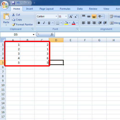
First of all, open an excel workbook and enter the data you want to compare.
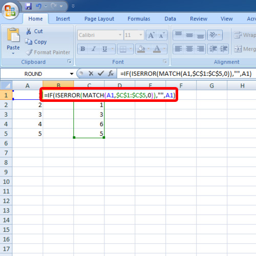
Once you have entered the data in multiple cells, we will insert the match function. Type in the following formula:
=IF(ISERROR(Match(A1,$C$1:$C$5,0)),“”,A1)

Step 2 – Explanation of the formula
In the formula, A1 is the cell that you want to compare. $C$1:$C$5 is the data range you want to compare A1 with. Empty inverted commas mean that the field will be empty when the cells don’t match. If the data in A1 matches the data in the cell range, then A1 will be written there.

Step 3 – Modify the formula
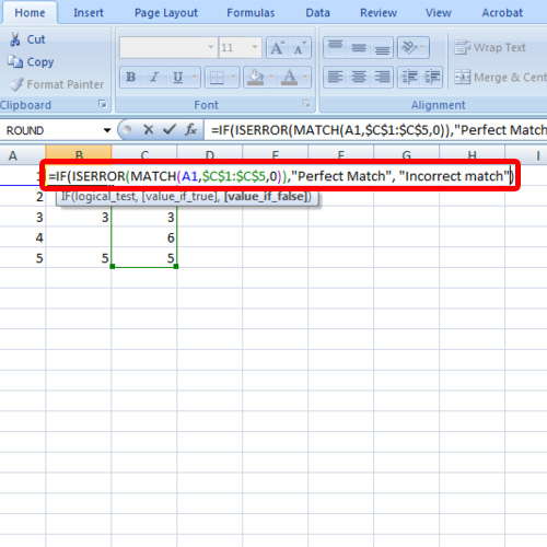
You can always modify the formula as per your requirements. Let us say that we want perfect match to be written when the cell matches the multiple cells selected.
In case of an imperfect match, we want incorrect match to be displayed. In order to do this, simply put imperfect match between the inverted commas of the formula.
Put perfect match in inverted commas at the very end of the formula. Perfect match would be written when the cell matches the data range we have inserted in the formula.

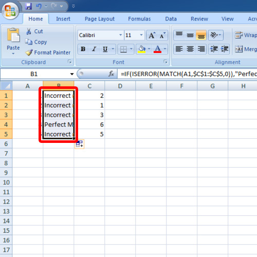
Step 4 – Drag the formula down
Drag the formula down to the cells below if you want to apply the formula to these cells as well. In this manner, you can compare multiple cells in Excel.

 Home
Home