In this tutorial, you will learn how to use the HLOOKUP function in Excel.
There are times when you want to calculate a value which resides in a separate table, but don’t want to use IF commands for this. Lookups, vertical and horizontal, provide you with just the means to do it.
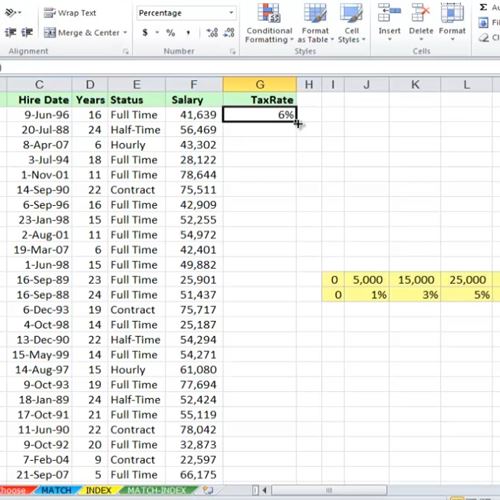
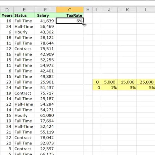
In our example, we have our Horizontal Table in the same spreadsheet, but it could easily be in a separate one, or even in a separate workbook. As you can see, the table is an index of tax rates according to the offered salary. If such rules change along the way, we will need only to modify the Horizontal Table.
Step 1. First, make sure the Horizontal Table is sorted in ascending mode. Then go to the first cell in the list that you want to calculate the lookup. Start typing:
=HLOOKUP(the value you search in the index comma the horizontal table comma the indexable row, in our case the row of percentages)

Step 2. Hit Enter. Excel will calculate the value by looking up in the entire Horizontal Table.

Result: Congratulations, you have learned how to use the HLOOKUP function in Microsoft Excel.
 Home
Home