In this tutorial you will learn to select, freeze and unfreeze a single or multiple rows using a specific function in the ribbon.
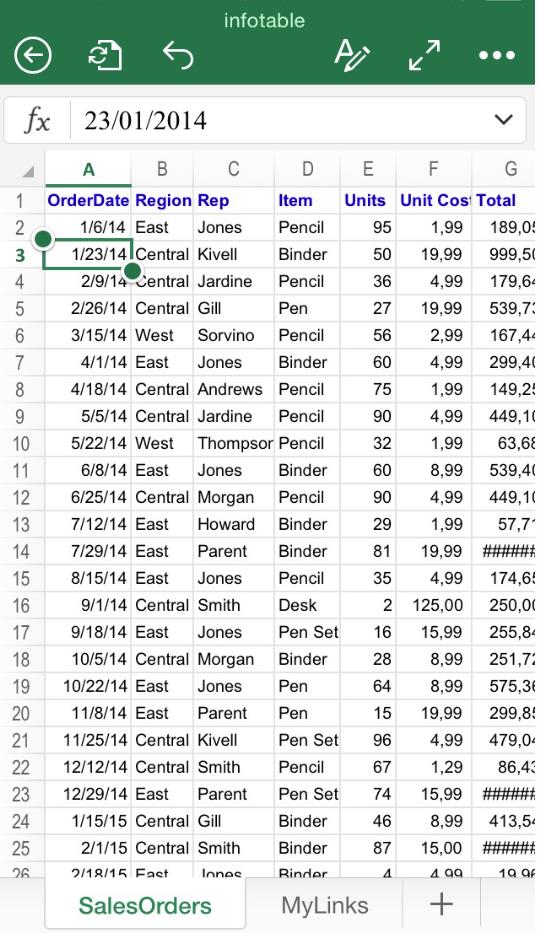
Step # 1 – Selecting the row / column you would like to freeze.
In this case, we will freeze the first row. To achieve this, the first step is selecting the row below the last row you would like to freeze:

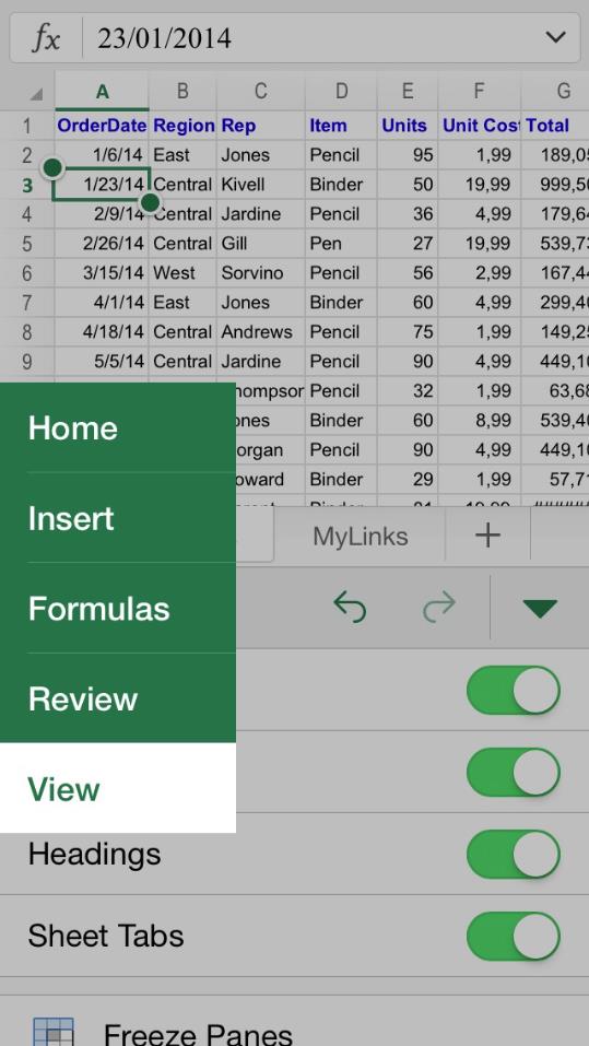
Step # 2 – Go to the “View” menu
You will have to click first the “ribbon” button as explained in previous tutorials.

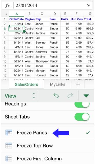
Step # 3 – Freeze function
Once inside the “View” menu, click the option “Freeze panes”. You will realize that a thicker line will appear automatically signaling the frozen row:

You will also realize that a “tick” will appear on the right side of the option “Freeze Panes”. To unfreeze the row, all you have to do is press again said option, making disappear the “tick” in the process.

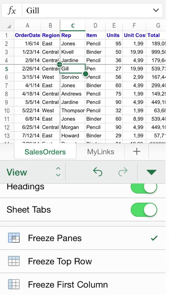
You can also freeze multiple columns and rows. Simply change the selection in the first step to cover a wider number of rows and/or columns, and then just repeat the rest of the steps in the same way. The screen should look like this at the end:

 Home
Home