In this tutorial we will be showing you how to join cells in Excel such that their data is combined into one cell which was previously present in two cells. People have a whole list of names of employees in their excel sheets. This can go up to several hundred or even thousands of rows. Suppose if you want to join or merge the data from two cells into one then it would take a lot of time. In order to do that you can use a formula that will do this step for you easily.
Follow this step by step tutorial to learn how to combine two Excel cells such that their data is combined into one.
Step # 1 – Insert a new column and write the formula
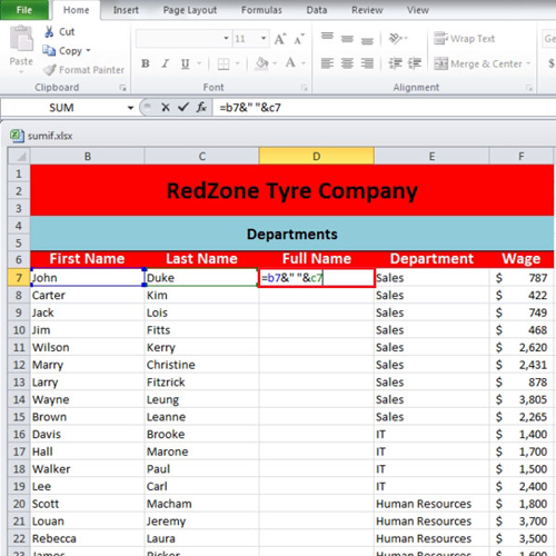
In this tutorial as you can see that this worksheet has the first names of people in column “a” and last names in column “b”. In order combine them first we will have to insert a new column after column “c”. To insert a column, select column “d” and right click on it. From the menu select “insert” and the new column will be inserted. Write the heading of “full name” in that new column then write “=b7&” “&c7” and press the “enter” key.

Step # 2 – Copy the data
When you press the “enter” key after writing the formula, Excel will combine both of the names. The formula can be explained by saying that we want Excel to get the data from cell “b7” and give a space before getting the data from “c7”. Use the “auto fill handle” to drag down till the end and when all the names have been combined select the whole column and right click on it. From the menu select the “copy” option.

Step # 3 – Paste the data as values
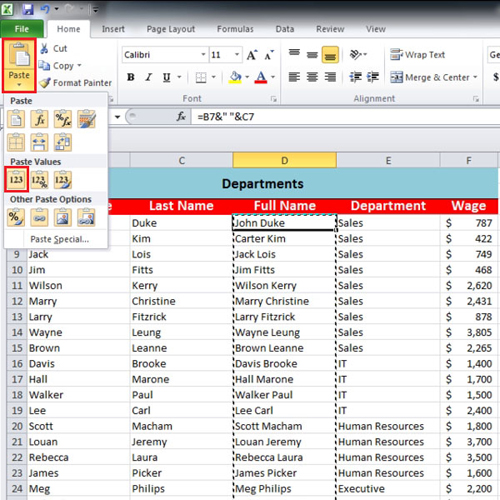
After you join cells in Excel and copy the data of the combined cell, click on the first cell of column “d”. This contains the name is the cell number “d7”. Go to the “paste” button which is situated on the upper left side of the screen. From the “paste” menu select the first option under the “paste values” heading.

Step # 4 – Delete the first two columns
We wanted to delete the first two columns but the names that were appearing to be as text were actually formulas and since they were getting the data from the first two columns it was necessary to first convert those formulas into values. After pasting, select the first two columns and right click on them. When the menu appears, click on the “delete” option and the columns will be removed.
As you can see from the above tutorial, it is very easy to combine two excel cells by joining their data into one.

 Home
Home