Microsoft Excel is a detailed software that can be used as a multiple analysis tool. It gives simple options that can help you manage and manipulate data to derive desired or actual results. It is important to understand the workings of this software to be able to use it effectively. You can create Custom View in Excel so that you don’t have to set your view each time you want to review a certain part of the Worksheet. It is very simple to create Views in Excel and you can have multiple views to suffice for each type. Follow this step by step to learn how to create multiple custom Worksheet views in Excel.
Step # 1 – Create View
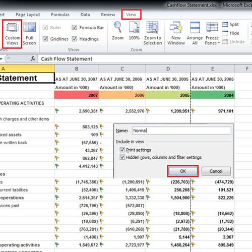
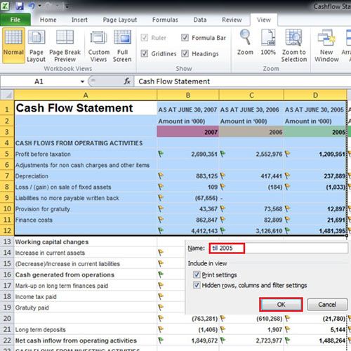
In order to create different views in Excel, go to the “View” tab and under the “Workbook Views” group, click on the “Custom Views” button. With that done, the “Custom Views” window will open up. Click on the “Add” button and give a name to this View.
Step # 2 – Add different Custom views
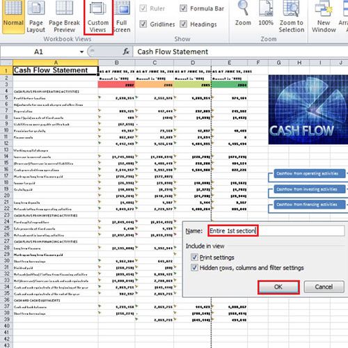
In this tutorial we have made multiple custom views in Excel. First of all we made the “Normal” view in the Excel Worksheet. Next, we zoom out the sheet up to 60%. This way, we can see the entire cash flow statement. Once done, we will create another custom view using the same steps.
Step # 3 – Access different views
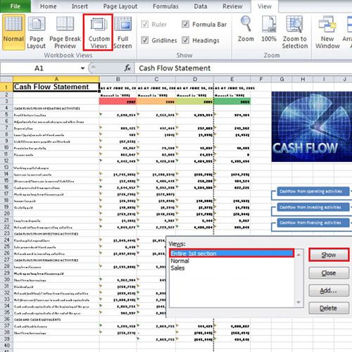
Now open the different views that we created to see if they work or not. To do so, move over to the “Custom View” button and in the window that opens, double click on the name of the view that you wish to open. You can easily access all the different custom views you create from here.
Step # 4 – Click on ‘Print Selection’
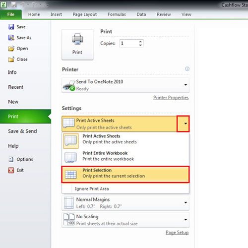
Under the Settings tab, click on the “Print Active Sheets” option, which is set by default, and select the “Print Selection” option. Now only the highlighted cells will be printed.
Step # 5 – Print particular views
Now when you select any of the Custom View and press ‘Ctrl + P” on the keyboard, only that particular selection is printed instead of the whole sheet.
 Home
Home