Scenario Analysis can better be explained as “What if” analysis. Each time you change a value you will get a new result. Scenarios in Excel 2010 can help you make and then save different values that give different results. The results can be categorized as “best case”, “worst case” and so on. In this tutorial we can see that there is a loan amount, interest rate and pay off period.
Follow this step by step tutorial to learn how to use scenarios in formulas in Excel.
Step # 1 – Click on “Scenario Manager”
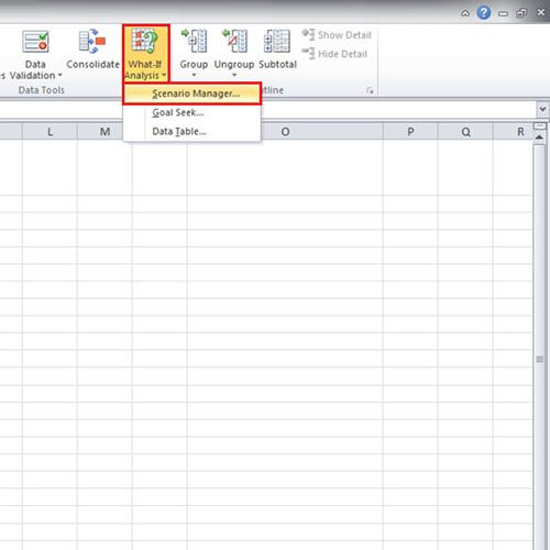
First of go to the “Data” tab and in the “Data Tools” group you will find “What If Analysis” button. Click on that button and from the drop down menu select “Scenario Manager” option.
Step # 2 – Add a scenario
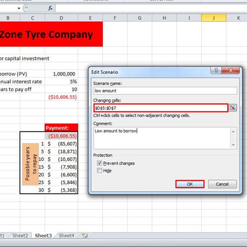
When you will click on the “Scenario Manager” option, the “Scenario Manager” window will open. Click on the “Add” button and “Add Scenario” window will appear. Give the Scenario in Excel, a name and from the “Changing Cells” section you will be able to select the range so select the range from cell “D5” till “D7”. You can add comments to the Scenario as well. When you are done, click on the “OK” button.
Step # 3 – Enter different values
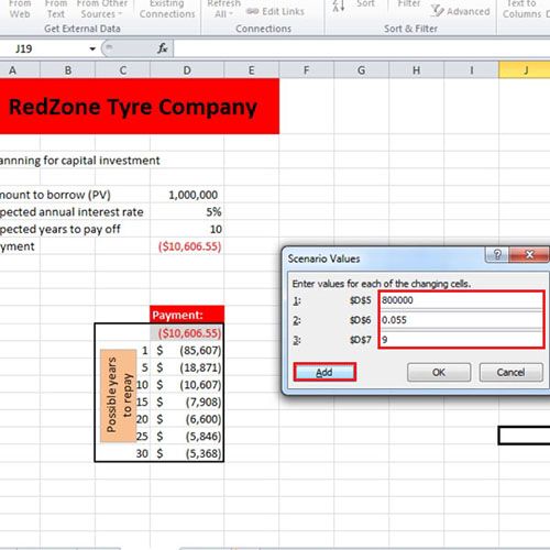
After you click on the “OK” button and a new box will open. We had previously calculated that if we take a loan of “One million dollars” and the exchange rate is “5%” and years to pay off are “Ten” then you will have to make a monthly payment of “$10,606”. This time we will say that what if we borrow a loan of “$80,000” and the interest rate has increased to “5.5%” and the time to repay has become “9 years”. After you input the data click on the “Add” button as 2 more scenarios will be added. The two scenarios are called “Original amount” and “High amount”.
Step # 4 – Click on the “Summary” button
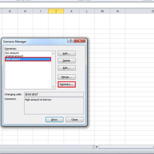
When you are entering the values of last scenario, instead of pressing the “Add” button click on the “OK” button and the “Scenario Manager” will open. Click on different scenario names and the values in the Excel Sheet will start changing. Click on the “Summary” button which is on the lower right side of the “Scenario Manager”. This is how formulas in Excel can be used for Scenario Analysis.
Step # 5 – Look at the Scenario Summary
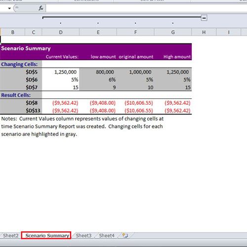
After you press the “Summary” button, “Scenario Summary” box will open. Click on the “OK” button and the scenario summary will be shown to you in a new sheet. You can have a quick glance for comparison in one go and you can give names to the “Changing Cells” as they will be represented by the cell reference.
 Home
Home