If you have entered data into an Excel sheet only to realize it would be better as a row rather than a column, or vice versa, then knowing how to flip the data is a valuable skill.
Step # 1 – Copying the Data
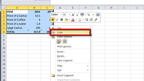
First off, load the sheet that has the data you want to flip. Here we have a small table about the price of some items. We want flip this so the price data is in a row, not a column. First highlight the table, right click on it and choose “Copy”.

Step # 2 – Using the Paste Special Window
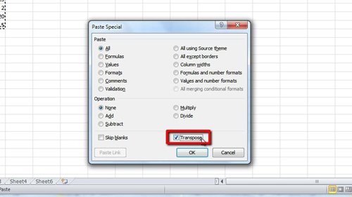
Now that the data is in the clip board, click where you want the new table to appear. Here we are placing it just right of the original table. Right click and navigate to “Paste Special…”, in the menu that appears click on “Paste Special…”. This will open a new window, check the “Transpose” check box at the bottom and click “OK”.
Step # 3 – Viewing the Transposed Data
The data will be inserted into the spreadsheet in the new location and as you can see all of the data has been flipped so that the prices are now in rows, rather than columns. This process will also work the other way round.

 Home
Home