HowTech

In this video tutorial we will show you how to create Excel chart with 2 y-axis or x-axis.

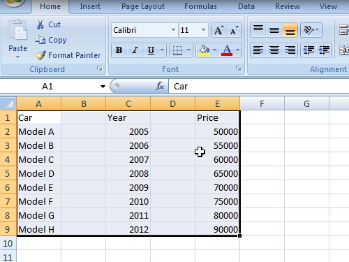
In order to create an Excel chart with 2 y-axis or x-axis, open your Excel document. Select the data in your document.

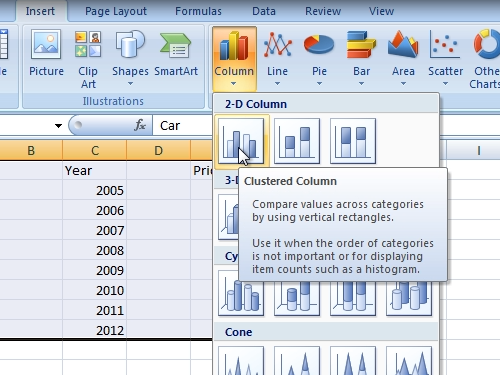
Go to the “insert” tab. Click on “Column” and choose “2-D column”.

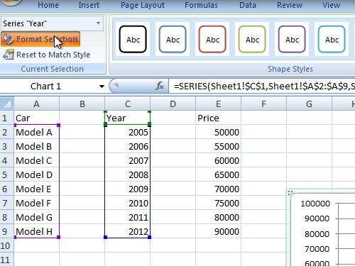
Select columns in chart with a mouse click. Go to the “Format” tab and choose “Format selection”.

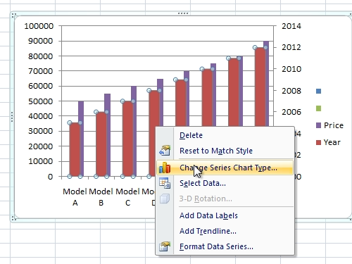
In the appeared window, choose “Secondary Axis” in “series Options”. After that, right-click on columns and choose “change series chart type”.

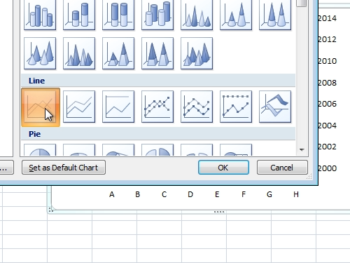
Select “Line” chart.

Now you know how to create a chart with 2 y-axis or x-axis in Excel.