In this tutorial, we will show you how to align data in Excel. There are several ways in which you can align data in Excel. You change the orientation of the text, format cells and increase or decrease indent. Furthermore, you can change the alignment of the text as well. We will also show you how to find unique items from large lists in Excel. Managing large lists can be a hassle. We will show you how to use a pivot table and find a solution to your problem by customizing the pivot table as per your requirements.
Step # 1 – Apply Merge & Center
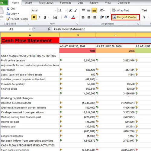
First of all, we will make use of the “alignment” group which can be found under the home tab. Select the cells that contain the heading and press the “merge and center” button. The heading will appear in all the five cells; however, they will not be five cells anymore but one cell as we have merged all of them together.
Step # 2 – Change orientation
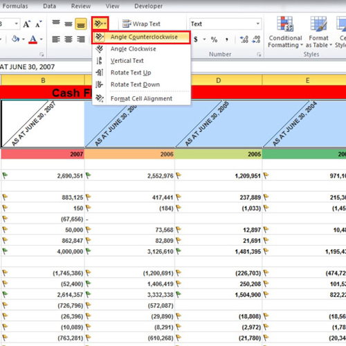
Now if you want to change the orientation of your text then select the cells, click on the “orientation” button and select the angle. In the tutorial, we have shown you how the text will appear if you choose the “angle counterclockwise” option.
Step # 3 – Format Cells
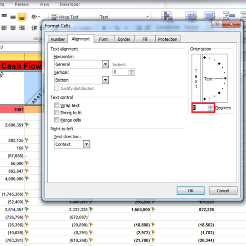
Another way to do so is by clicking on the “format cell alignment” option in order to open the “format cells” box. You can make your custom orientation by adjusting the degrees; we have changed it back to normal by selecting “0” degrees.
Step # 4 – Increase or Decrease Indent
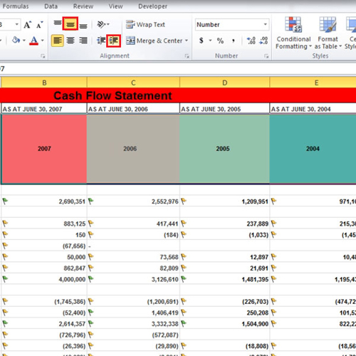
If you want to increase or decrease the indent of your text, first select the orientation and then click on the indent button to change it. You can also choose the “top align”, “middle align” and “bottom align” buttons to do it. If your data is being displayed horizontally, the indent buttons will make your text move rightwards or leftwards depending on which one you press.
Step # 5 – Apply Justify to text
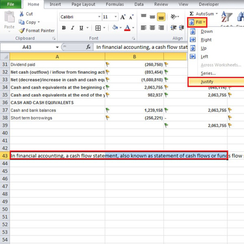
If you have imported text from somewhere and pasted it, then it will be pasted in one cell and stretched horizontally. You’d have to scroll rightwards to read it. After selecting two to three cells, click on the “fill” button. From the drop down menu, select the “justify” button and the text will appear in those cells which you have selected. Make sure that the cells below are empty so that the text does not overlap any other data. If you want your text to appear vertically, then select the cells and click on the “justify” button again. These were some of the different ways in which you can align data in Excel.
Step # 6 – Insert Pivot Table
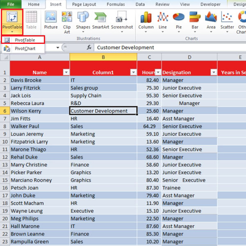
The next thing is displaying unique items from large lists in Excel. First of all, go to the insert group and click on the “table” option. When the “create table” box appears, click on the “ok” button. Then from the insert tab, select “pivot table” from the drop down menu. A new box will appear; click on the “ok” button and the pivot table will be created in a new sheet.
Step # 7 – Customize Pivot Table
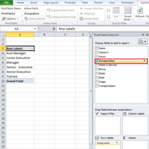
On the right hand side of the screen will be our “pivot table field list”. If you want to sort your data according to the states and rate, then check both of them. You can add wages and other fields to it as well or simply checkmark them one at a time to see the unique entries of any field. In this manner, you can work with large lists in Excel.
 Home
Home