In this tutorial you will learn how to create a drop-down menu in Excel
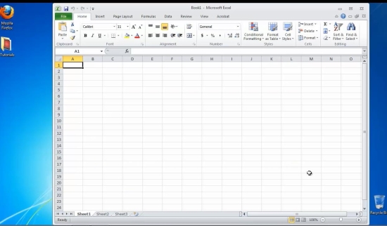
Step 1. Open your Excel workbook.
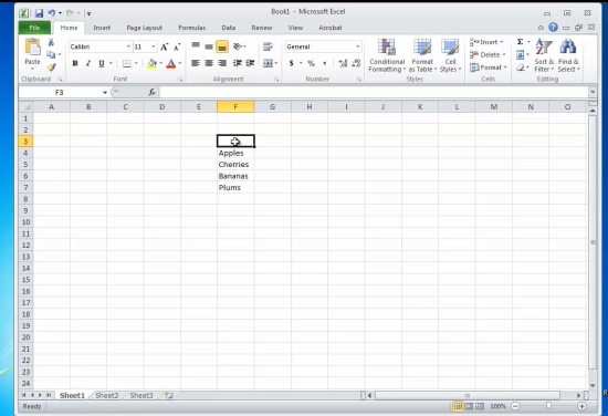
Step 2. On a separate sheet, create the list of options that you want to be displayed in the drop-down menu.
Step 3. Select the entire area of options, right-click and choose “Define name”.
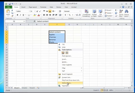
Step 4. Name your list of options, let’s say: “ValidEntries”.
Step 5: Go to the sheet where you want to display your drop-down menu. Select the cell that will contain it.
Step 6: From the Data menu, choose “Data Validation”, then “Data Validation”. You are presented various validation criteria.
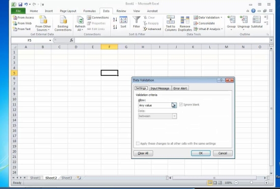
Step 7: The one that we need is called ‘List”, as it is the list of options we want the user to have.
Step 8: Make sure in-cell dropdown is marked on.
Step 9: At the source, put the sign “=” and the name you’ve defined, in our case “=ValidEntries”.
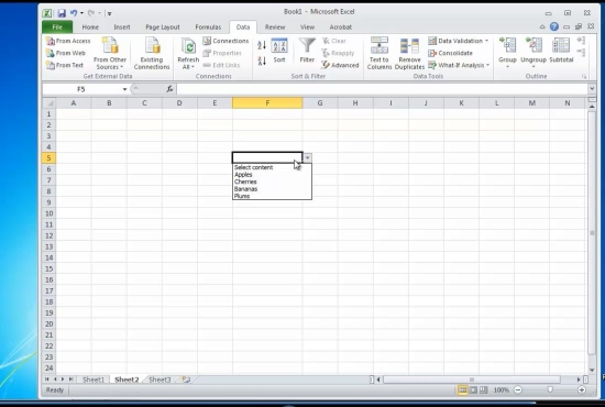
Result: Your cell now displays a drop-down menu of selected values. Congratulations! Now you know how to create a drop-down menu in Excel.
 Home
Home