In this tutorial you will learn how to create pivot table in Excel.
A pivot table is a particular format of table specific to Microsoft Excel, which will allow you to see a bird’s eye view of a table without you having to create formulas for calculations. It is called pivot table because you can easily alter its layout and structure, regardless of the data it feeds from.
Here is how to create one.
Prerequisites: Microsoft Excel.
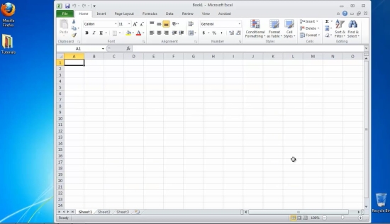
Step 1. Open Excel and go to your spreadsheet. Make sure you have different columns of data with their names labeled on top of their fields.

Step 2. Position your cursor on where you want your Pivot Table to appear.

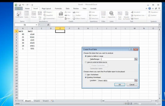
Step 3. From the Insert Tab, the Tables subsection, click on Pivot Table. A menu appears.

Step 4. Select the entire range of data you want to be included in the reporting of the Pivot table, including headers.
Step 5: Mark “Use an external data source” if your values were processed by a non-excel application, otherwise leave that field empty.
Step 6: Choose “New Worksheet” if you want the Pivot Table to be placed in a separate worksheet, otherwise choose Existing.
Click OK.
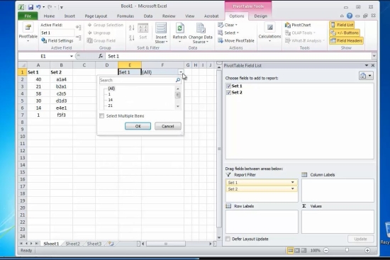
Step 7: The right side of your Excel pane is now split into two types of fields: the upper one shows your sets of data, and the lower one has four drop zones of reporting. Depending on what you want to summarize from your table, you drag and drop the contents of the upper part into one of the four drop zones of the lower part.

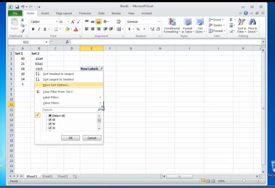
Step 8: Experiment with the looks and the results until you are happy with the outcome.

Result: Congratulations. You have learnt how to create a pivot table in Excel.
 Home
Home