Macros are scripts that you record; certain actions you may perform in a specific sequence. You might have to perform a set of actions in a particular order on a day to day basis. Instead of doing it manually, do it just once when recording the macro. Next time you want to perform those set of actions, simply run the macro.
In this tutorial, we will show you how to edit a macro in Excel. We will work with a macro we have already made. We will make some changes to it in order to guide you how to edit your macro for yourself.
Step # 1 – Click on the Macros button
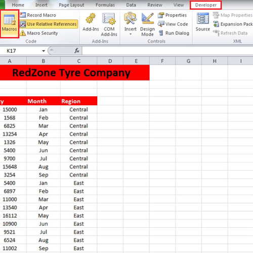
First of all, open the workbook from which you want to retrieve the data, then switch your workbook and return back to the previous one. Go to the “developer” tab and click on the “Macros” button over there.

Step # 2 – Edit Macro Option
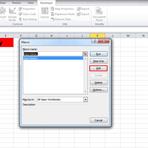
In order to edit macro in Excel, click on the “edit” button when the “macro” window opens.

Step # 3 – Make changes to the Macro code
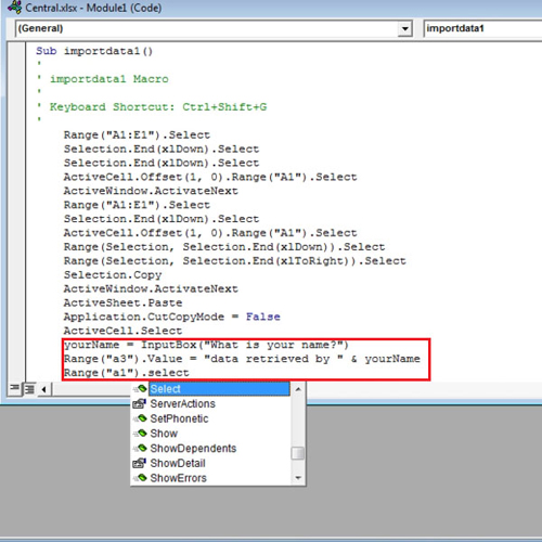
A new window will open of “vb editor” where you can add codes. Go to the bottom of the codes. The words “end sub” mean that it’s the end of the codes. So we have to write the code before “end sub”. Click at the end where it says “active cells dot select” and press enter a few times to add space. We already made a macro which helped us in retrieving data from other workbook. Now we want to edit the macro by inserting a code such that the Macro will ask for the name of the person when the macro is run. In order to do so, write
yourname “ InputBox (“What Is Your Name?”)
range(“a3”).Value = “data retrieved by ” ampersand yourName
range (“a1). select
The first code is for asking the question and displaying it in a box. The second code tells it where to appear and what should be written before the name. The final code automatically selects the first cell.

Step # 4 – Run the Macro
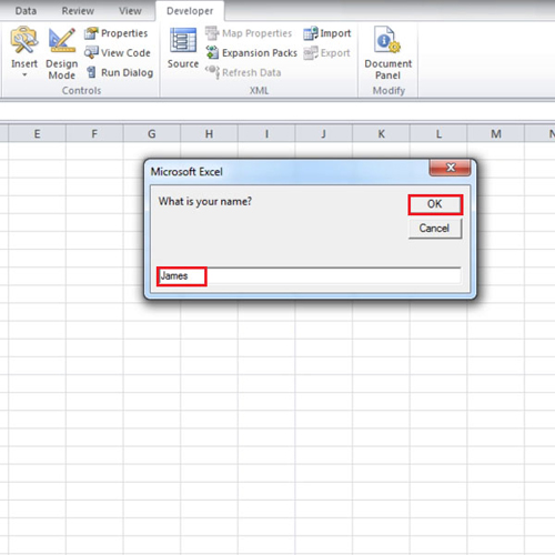
Now when you will press “ctrl + shift + g” which is the shortcut key to run the macro, it will get the data and will ask you for your name. Enter the name and press the “ok” button. In the tutorial, you will see that in cell “a3”, which we had used in the code, “data retrieved by james” will be displayed. Cell “a1” will automatically be selected.

 Home
Home