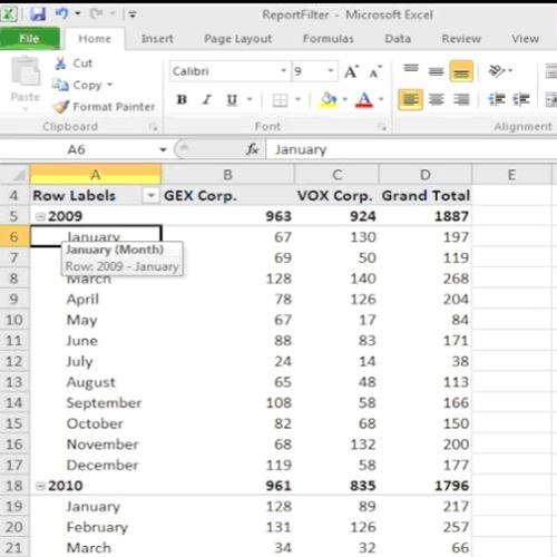
In this tutorial, you will learn how to sort data in a Pivot Table.
In Excel, you can limit the data displayed in a Pivot Table by applying one or more Filters to it without affecting the design of the table.
Step 1.
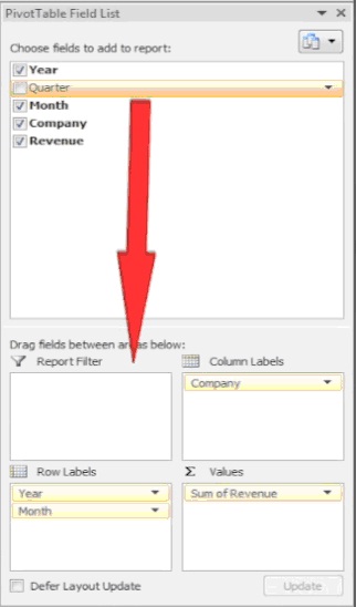
To do so, click anywhere inside your Pivot Table to activate its controls, then add your filter at the Report Filter tab in the lower right pane.

Step 2.
In our case, we will filter the whole Pivot Table by quarterly results. Drag the Quarter field from the Pivot Table list pane to the Report Filter tab.

Step 3.
Excel will ask you if you want to replace the current filter, which is the default one created in the first cell at A1. Agree to do so and Excel will create for you a filter area.

Step 4.
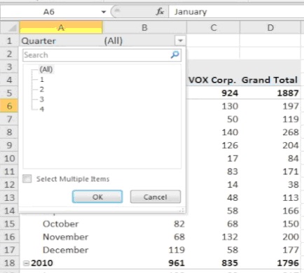
Click on the filter box in the cell near Quarter to filter on-the-fly.
Checkmark Select Multiple items before you create your selection to for complex filter results.

Step 5.
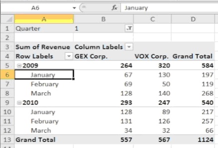
Click OK. Excel brings you the updated results.

Result: Congratulations, you have learned how to sort your data in a Pivot Table.
 Home
Home