In this tutorial you are going to learn how to hide worksheet Excel. This tutorial has been made on Excel 2010 and applies to this versions, as well as 2007.
Step # 1 – Navigating to the Sheet you Want to Hide
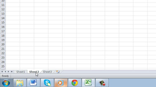
As you can see here we have a spreadsheet open with the default three sheets available that can be accessed from the bottom. First you need to click on the one that you want to hide, here we are choosing “Sheet 2”. You will be taken to that sheet.

Step # 2 – Hiding the Sheet
Now, make sure that you are in the “Home” tab from the options at the top. In the “Cells” area below this click on the “Format” icon. A menu will appear and you need to navigate to “Hide & Unhide”. Click the “Hide Sheet” option to hide the current sheet. It will disappear from the spreadsheet and you will be moved onto the next available sheet, in this case that is “Sheet 3”.

Step # 3 – Making the Sheet Visible Again
Now we are going to look at how to make the sheet visible again. Click the “Format” icon again and go back to “Hide & Unhide”. This time click the “Unhide Sheet” option. A dialog box will appear and it will list any sheets that you have hidden, here we can see that that is “Sheet 2”. Click “OK” and the sheet will once again be visible in your spreadsheet and that is how to hide worksheet Excel and then make it visible again.

 Home
Home