Excel provides its user with excellent sorting options. You can filter your data in Excel as per your requirements. Sorting in Excel allows you to re-arrange data as per your needs. In the tutorial, we will show you how to filter data according to multiple criteria.
In this tutorial, we will teach you basic and multi-field sorting in Excel.
Step # 1 – Use the Sort & Filter option
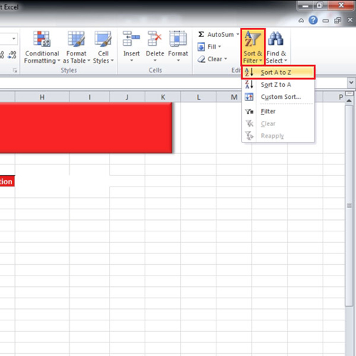
If you have a large data and you want to sort it in Excel, you can use the “sort and filter” option available in excel. In this tutorial, we will sort the data according to the departments. Click anywhere in the department column and go to the “editing” group and click on the “sort and filter” button. From the drop down menu, select the “A-Z” option. The departments will be sorted accordingly. Similarly, if we want to sort the data in the “hours” column, we will click on the same button and choose an option. In this case, the option is “from largest to smallest” because the column has numbers in it so the options will be given accordingly as well.
Step # 2 – Custom Sort
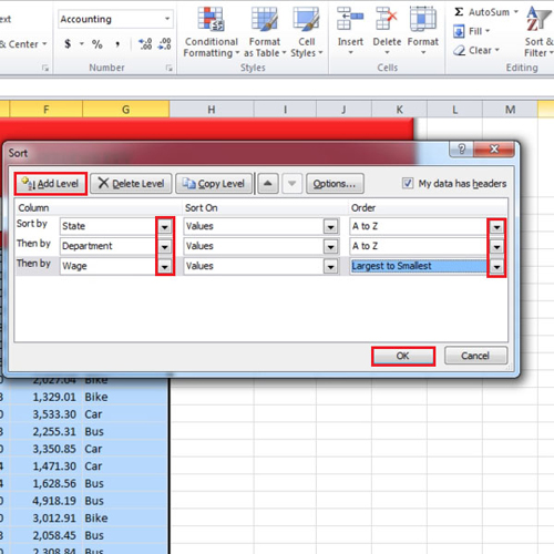
You can even customize how you want to sort. Click on the “sort and filter” button and choose the “custom sort” option. A small box will open. In this tutorial, we will choose to sort by “state” and apply order from “A-Z”. Now let’s add another level to it. Click on the “add level button” and in the “then by” field, select “department”. We will add another level and this time the criteria would be to sort by “wage”. Once done, we will click on the “ok” button.
Notice that the state of “California” is listed at the top and fulfills our sorting criteria requirements at all levels.
Step # 3 – Filter Option
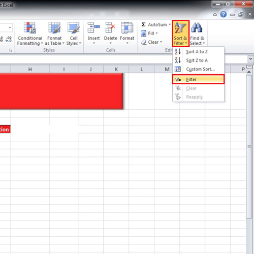
You can apply filters in Excel as well. Simply go to the “sort and filter” button and select the “filter” option. You will see that in the top row of the data there will be drop down filter buttons.
Step # 4 – Filter by specific field
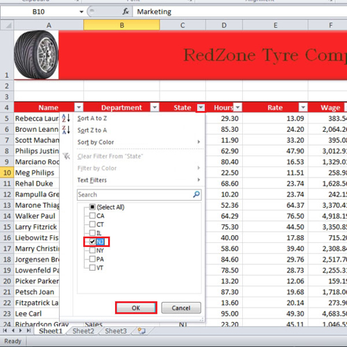
If you want to filter the data by “state”, click on the “state” button. Deselect all the states and then click on the state which you want to filter by. If you want to remove the filter then click on the drop down button and select the “clear filter from” option.
Step # 5 – Use Number Filters Option
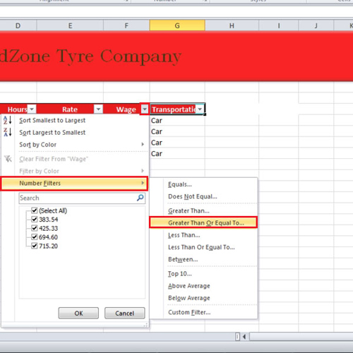
Next, we will filter our data on multiple levels. Consider you want to know the people who are in some specific department such as “Executive” and whose salary is more than five hundred. Apply the filter to the “department” column and select the desired department. In the wage column, click on the drop down button, go to “number filter” and click on the “greater than or equal to” option. Now write down the value you want to filter by and click on the “ok” button once done. This is how you can filter data in Excel with multiple criteria.
 Home
Home