In this video tutorial we will show you how to make an excel histogram.
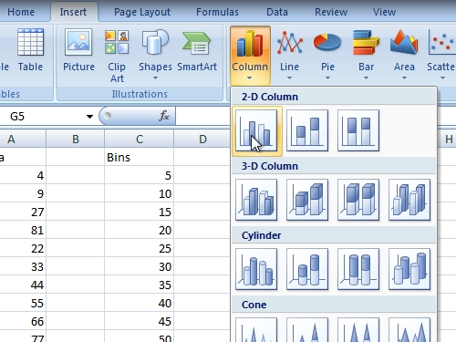
In order to create an excel histogram, open an excel document. Enter data into the cells. Then go to the “Insert” tab. Click “column” and select 2-D column.
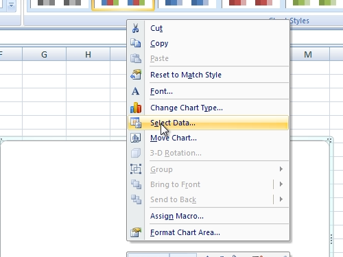
Then right-click on the created chart and click “select data”.
Select the data you want to add. Then in the “Select data source” window press “Edit”.
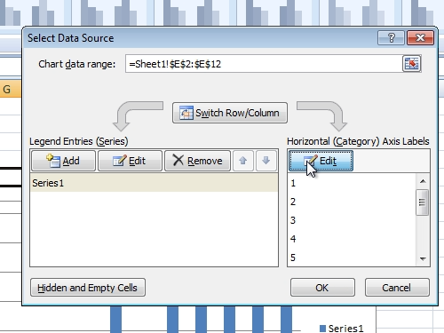
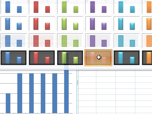
Select the data that must be added to the “axis labels” and click “ok”. Then press “ok” to close the window. Select the legend text on the right and press “delete” key. Then go to the “Design” tab and choose another chart style among “Chart Styles”.
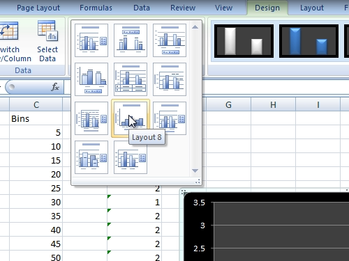
When done, go to the “Chart Layouts” and choose “layout 8”.
Then right-click on the left axis and select “Format axis”.
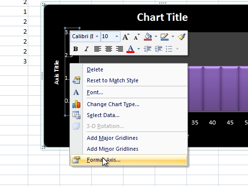
In the appeared window change the “major unit” and “Maximum” options. Enter the bottom and the left titles. Now your histogram is ready. Save the document.