Sorting data at times can be a huge problem when you have so many rows and columns and so much of data in them. Excel allows you to sort data the way you want. You will have a lot of choices as to how you want to sort it. For example you can classify your data according to the departments. Sorting data in Excel can be done easily by inserting a table. Even more you can delete duplicate entries in Excel after you add them in a table.
Follow this step by step tutorial to learn how to use tables in Excel to sort and filter data.
Step # 1 – Insert the table
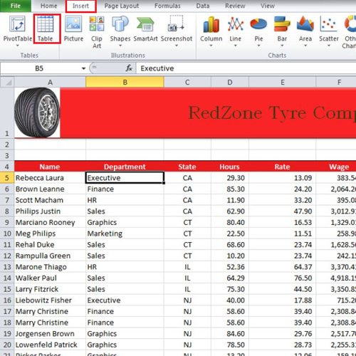
As you can see that in this worksheet we have 7 columns which consists of names, departments, states, hours worked, rates, wages and “transport”. Go to the “insert” tab and click on the “table” button. A small box will appear which will tell you the range. It automatically guesses the “range”. However, you can select the range yourself as well. Click on the “ok” button and the table will be inserted.
Step # 2 – Sort the data
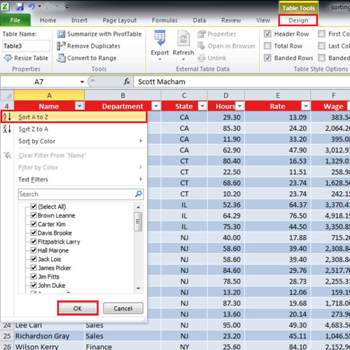
After the table has been inserted we can sort the data easily. Suppose we want to see if there has been any duplication in the data. Click on the dropdown menu of the “name” column and select the “sort A to Z” option. By default all of the filters will be selected but you can deselect them all and choose the one you want to sort the data.
Step # 3 – Find the duplicate entries
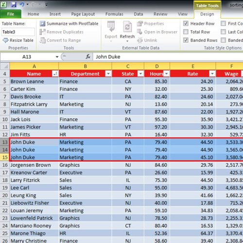
When you select the “Sort by A-Z” option then all the names will be sorted from A to Z. Scroll down and you will see that the name “john duke” is there three times and this is because the rate is not the same. If you scroll down further you will notice other duplicate entries as well like “Marry Christine” and “Wilson Kerry”. These entries are pure duplicates of each other.
Step # 4 – Remove Duplicate Entries
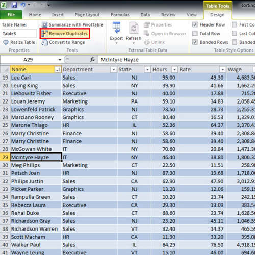
To delete the duplicate entries in Excel click on the “design tab” that appears when you click anywhere within the table. When you are in the design tab under the “tools” group you will find a button named as “Remove Duplicates”. Click on the button to remove these duplicate entries.
Step # 5 – Click on the “ok” button
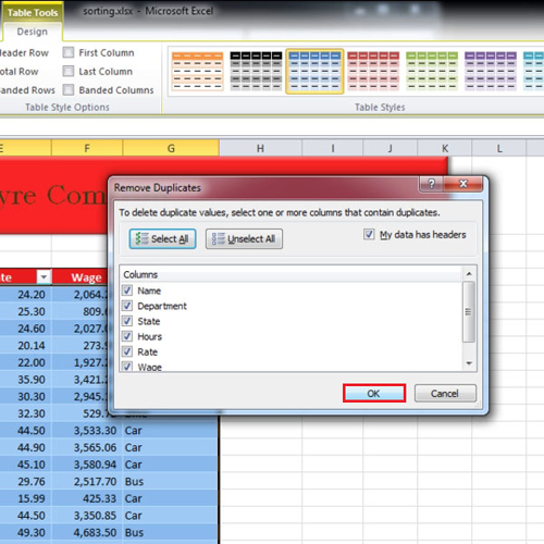
When you will click on the “Remove Duplicate” button a new box will open. From this box you will be able to select the criteria for deleting the duplicates. All the check boxes are marked by default so click on the “ok” button.
Step # 6 – Select the criteria
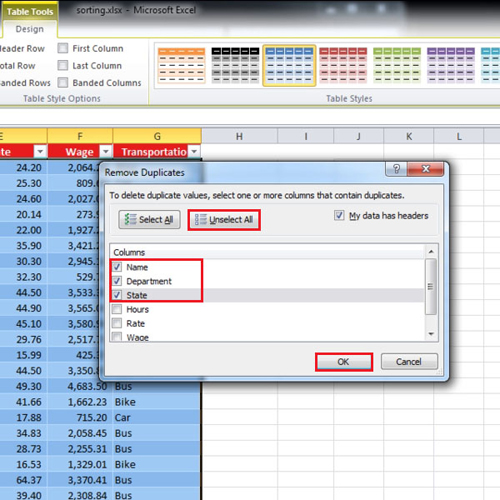
After you press the “ok” button, all of the duplicate entries will be deleted from the tables in Excel except for the “John Duke” one. This is because the last time we had selected all of the criteria or selected all of the columns which had duplicates in them. This time when you press the “remove duplicate” button, click on the “unselect all” button and choose the top three options only. Press “ok” once you are done. The duplicate entries will be deleted and a small notification box will appear which will tell you about the number of duplicates that were deleted.
 Home
Home