HowTech

Microsoft Excel is a detailed software that can be used as a multiple analysis tool. It gives simple options that can help you manage and manipulate data to derive desired or actual results. It is important to understand the workings of this software to be able to use it effectively. There are many more options in Excel with respect to using formulas. One of the most useful tools are the ability to trace in Excel where all your calculations are coming from or going to. Trace dependents in Excel or precedents so that you always know how values are come to. To learn how to apply such techniques, follow this step by step tutorial.

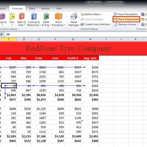
Step # 1 – Select ‘Trace Dependents’
To learn how to trace dependents in Excel, we have calculated the total and average for each group separately and then for both of them collectively. So basically all cells in this sheet are connected with each other. To know which cell is connected to what, you can use the “Trace Precedents” and “Trace Dependents” options. In this image you can see that the dependents have been trace showing the row adding up to totals and the column adding up to a total.

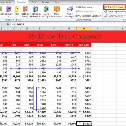
Step # 2 – Click ‘Trace Precedents’
Click on the “Trace Precedents” button to show which cells are contributing to the calculation in Cell E19, which are shown as cells E13 to E18.

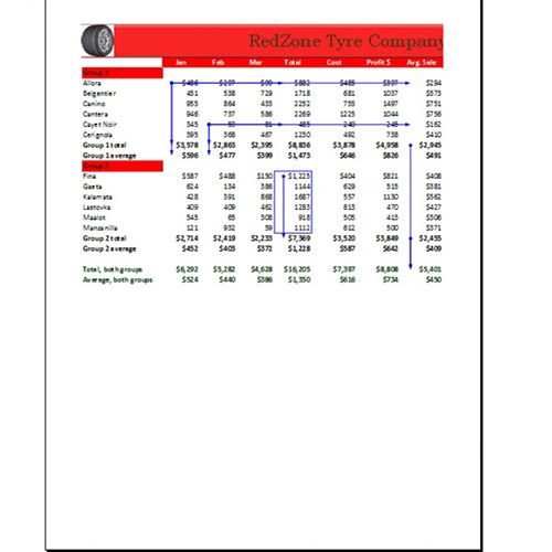
Step # 3 – View ‘Print Preview’
You can Print these precedents and dependents arrow as well. Notice how they appear in the Print Preview.

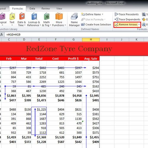
Step # 4 – Select ‘Remove Arrows’
If you want to remove these arrows, go to the “Formula Auditing” section and click on the “Remove Arrows” button.

Step # 5 – Press ‘Ctrl+Shift+]’
If you want to select all direct and indirect dependent cells then press “Ctrl + Shift + ]”.

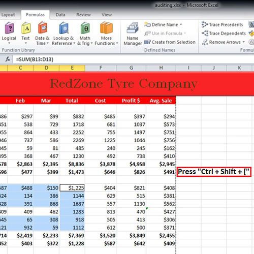
Step # 6 – Press ‘Ctrl+Shift+[‘
You can also use the shortcut key “ctrl + shift + [“ to select direct and indirect precedents.

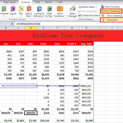
Step # 7 – Use ‘Error Checking’
If you remove some of the data from the sheet, the cells which were dependent on other cells will start showing errors. Click on any error, move over to the “Formula Auditing” section and click on the “Error Checking” button. From the drop down menu, select the “Trace Error” option. With that done, you can see that the values of cell B13 to D13 were being used to calculate cell “H13”. You can trace in Excel out all the errors by using the “Trace Error” option.