In this tutorial, we’re going to show you how to use the VLOOKUP function in Excel.
In this example, I have a list of people who have purchased Units, and a corresponding column of how many. I also have a column of people who have received those Units.
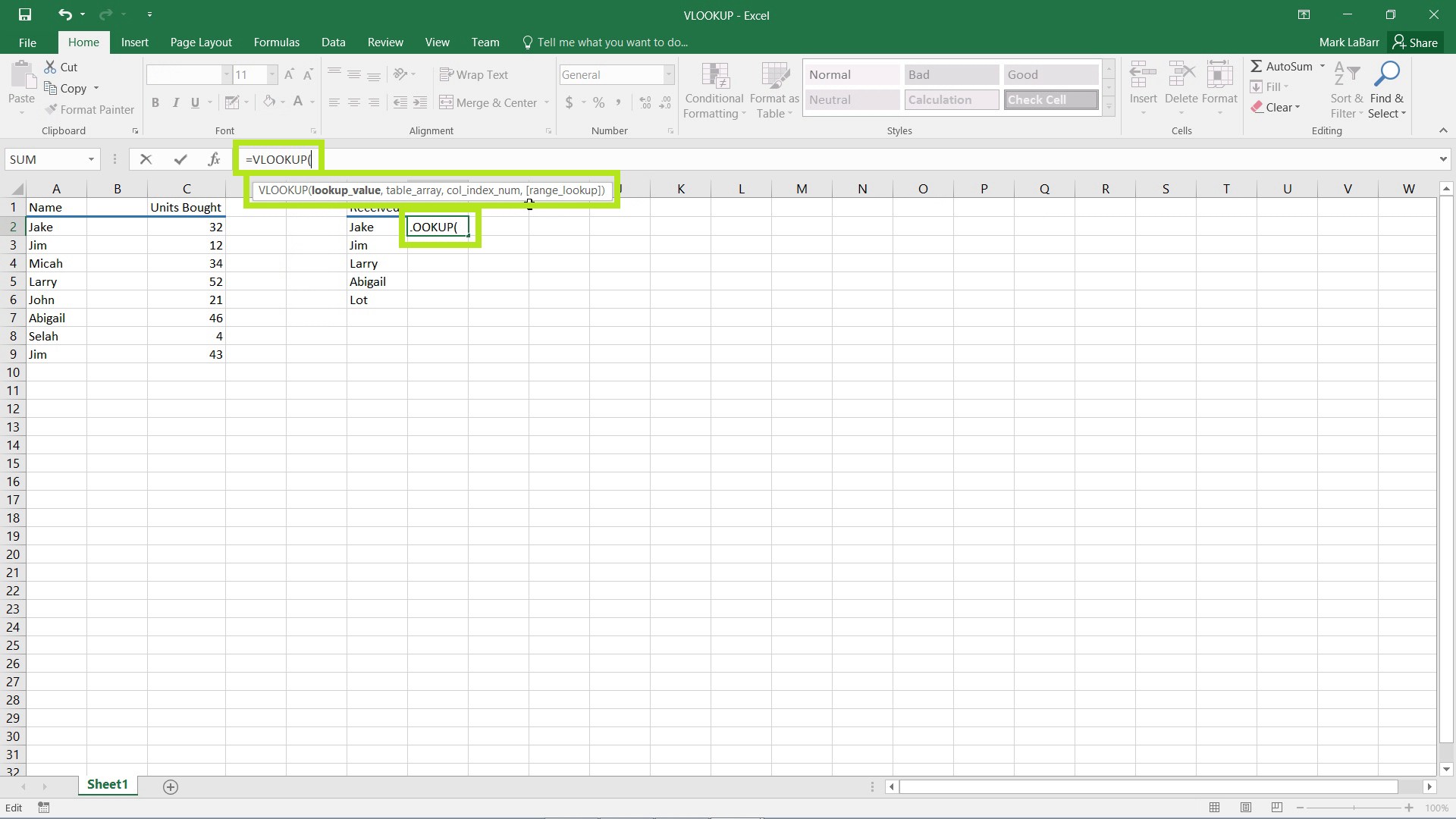
To get started, click on the cell you want to use VLOOKUP and type “=VLOOKUP(“ (without the quotes, just like in the example).
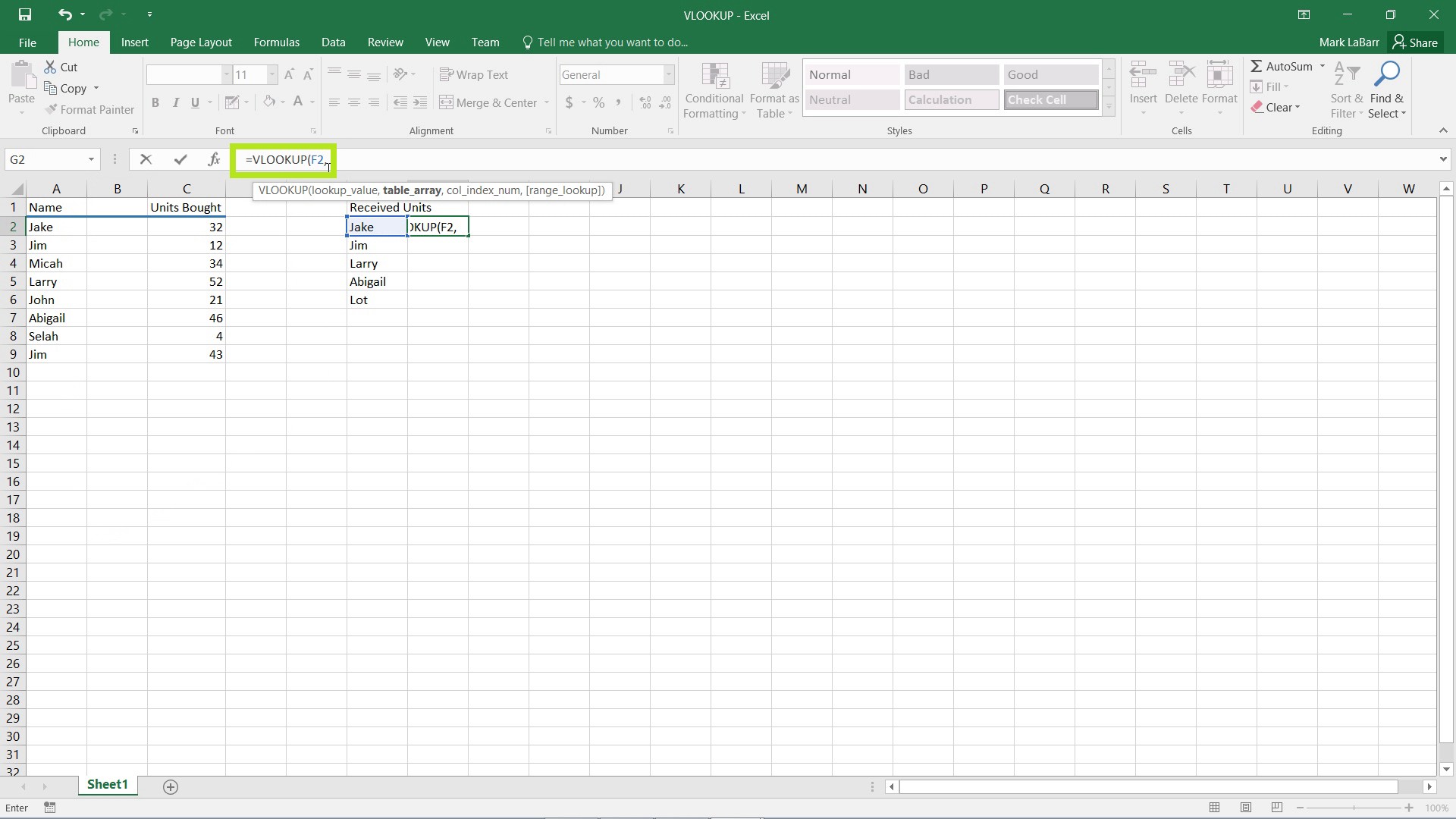
You will see by the tooltip for VLOOKUP that we need a lookup value. I will use the name just to the left of the VLOOKUP cell. The lookup value is the value that will be searched for in another later-specified column of values.
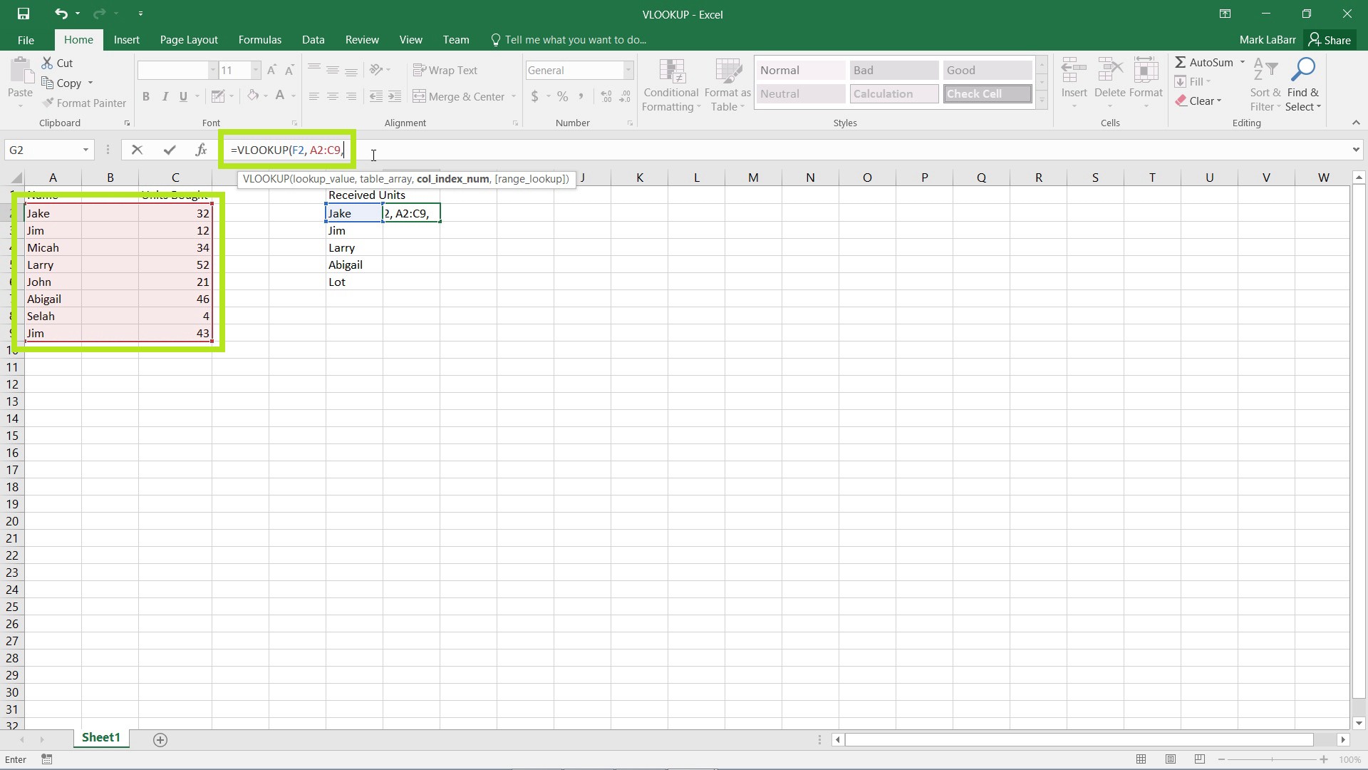
The next parameter is the table array we’re going to use to search for our lookup value. This table array in the first three columns I have for those who have bought units. Simply highlight that block of cells, disregarding the title/header cells.
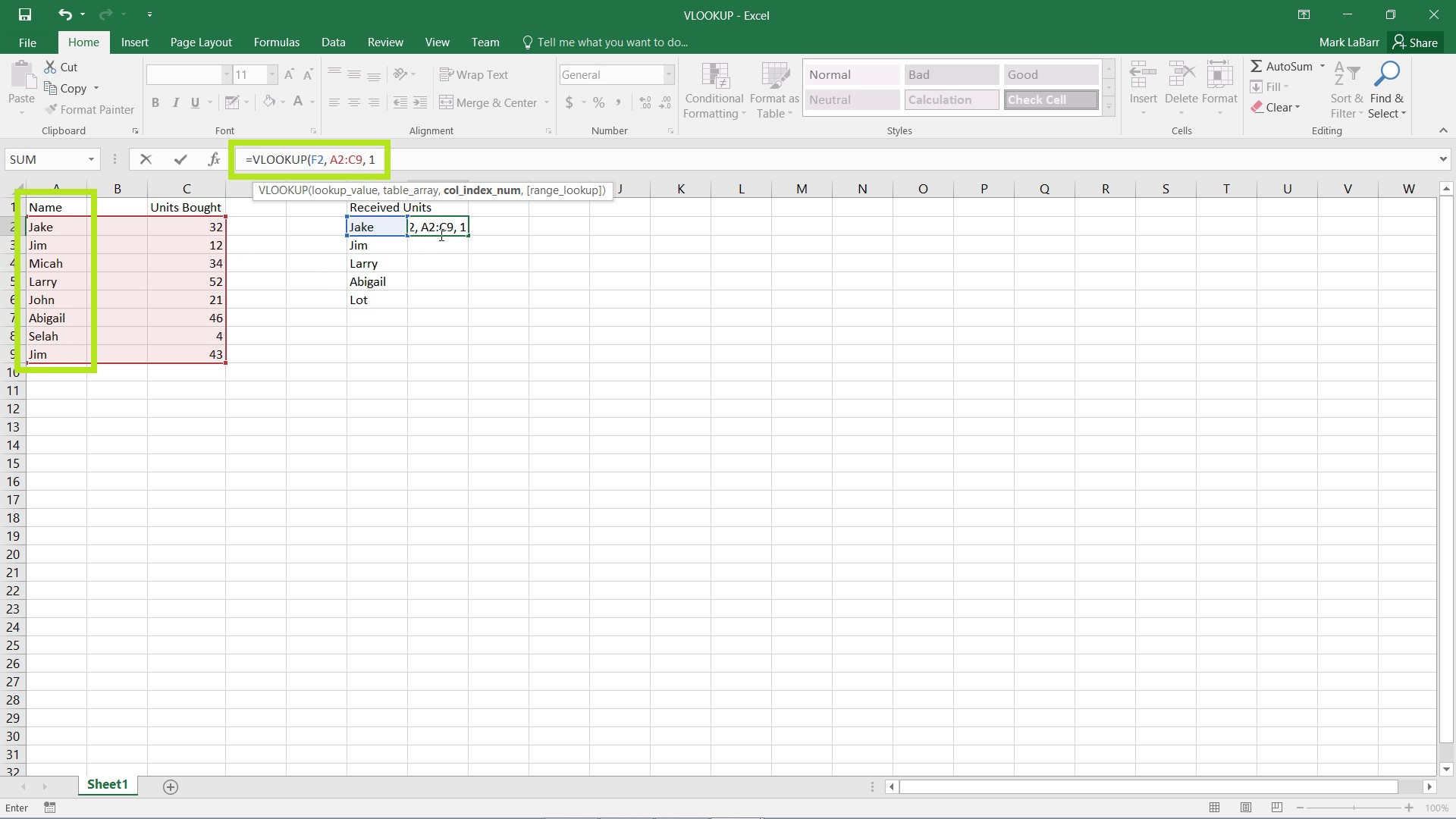
The next parameter (as bolded now in the tooltip) is the column index number. This will tell VLOOKUP the value from which column to output. For example, if Jake is found in the table array, should VLOOKUP output “Jake” in column 1, nothing in column 2, or “32” in column 3? For this example, I want VLOOKUP to output Jake which would be in column 1. Simply place a “1” (without quotes).
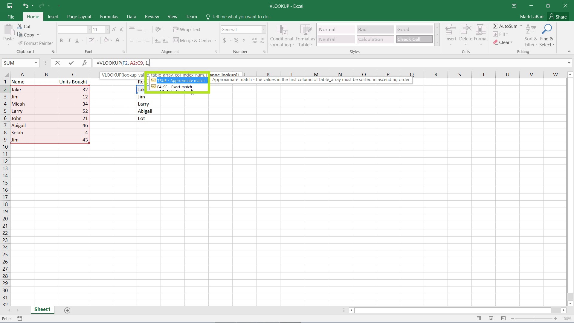
The final argument for VLOOKUP is the range lookup. It takes a true or false value. Putting TRUE has VLOOKUP look for an approximate match of the lookup value. Putting FALSE looks for an exact match. For this example, I want an exact match.
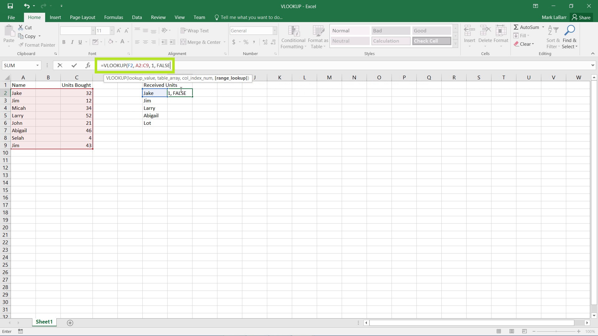
Simply type “FALSE” (without quotes). Or click it in the toolbar that pops up.
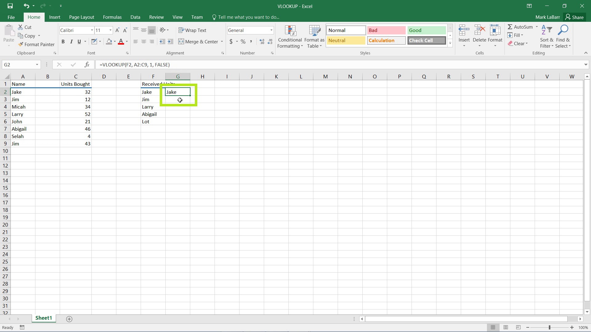
The final formula looks like this without the quotes: “=VLOOKUP(F2, A2:C9, 1, FALSE)”. Finally, press enter. The value “Jake” shows up in the cell because Jake was found in the table array and the column index number was set to output the first column.
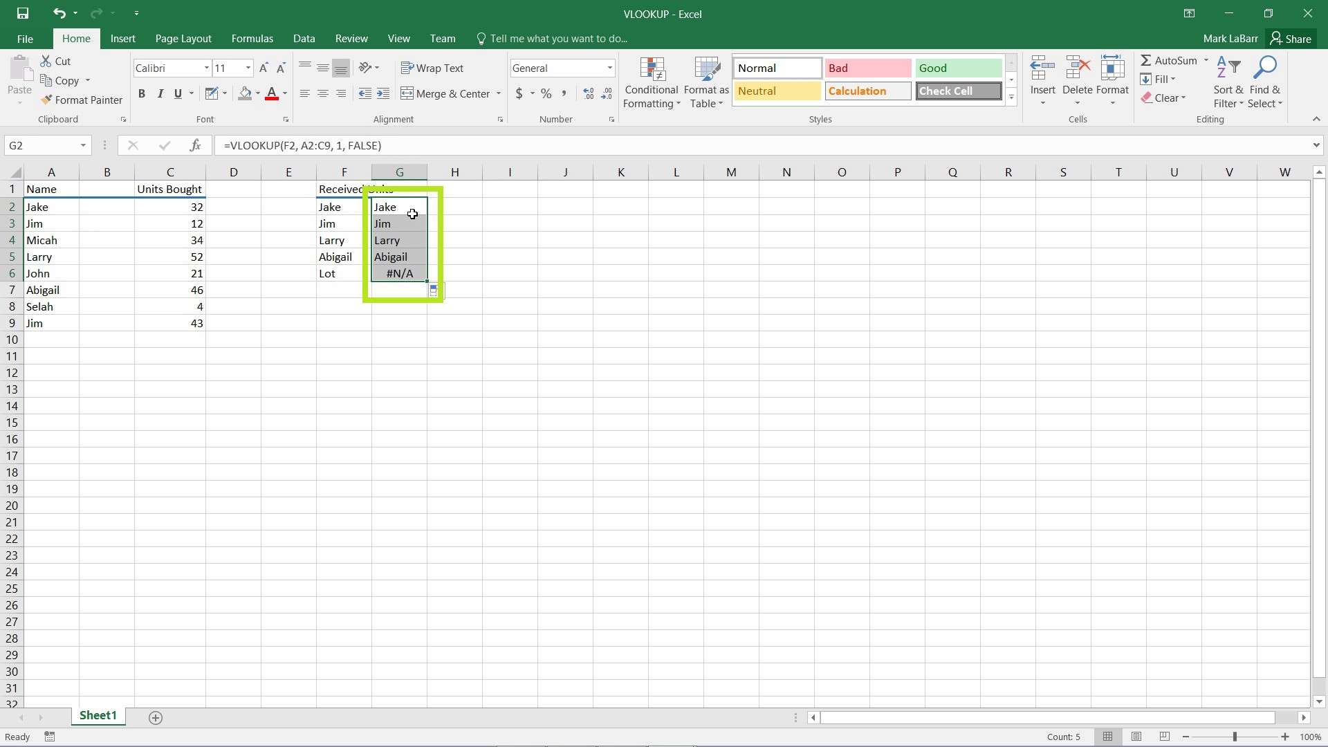
Click and drag the square in the bottom right of the selected cell to bring the formula down to the other cells. The names output, except Lot’s which outputs an error. This is because Lot is not in the list who bought units, but he received units.
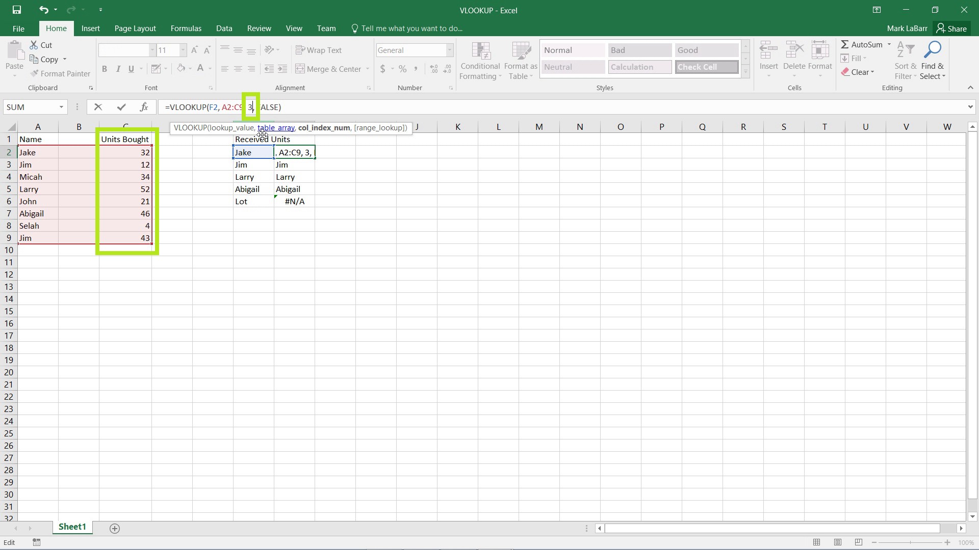
If we wanted to change what VLOOKUP outputs in the cell, change the column index number to a different column if available.
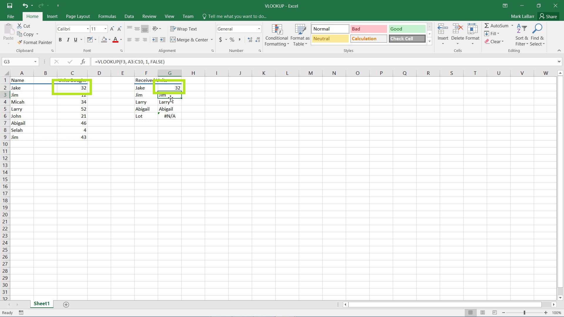
The cell now outputs “32”, the value in the third column of the table array.
 Home
Home