A confidence interval is a useful data analysis tool in Excel, this tutorial will show you how to construct one.
Step # 1 – Accessing Data Analysis
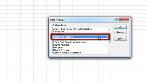
Start Excel and load the data that you want to create a confidence interval from. Here we have a column titled SMS, which indicates the number of text messages sent in a single day by a class of students. Click on the “Data” tab and on the right click on “Data Analysis”. In the window select the “Descriptive Statistics” option and click “OK”.

Step # 2 – Setting up the Data Analysis
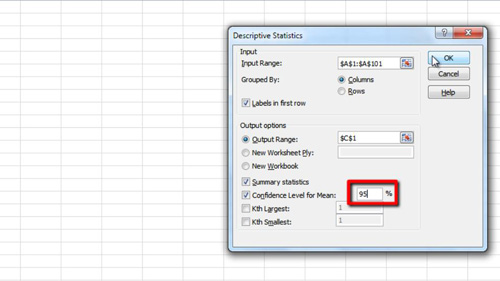
In the window that appears click on the “Input Range” box and click back to the spreadsheet and highlight all the data, including the column heading, here it contains 101 items, including the heading. Make sure “Columns” is selected and the “Labels in first row” box is checked. Click in the “Output Range” box and choose a cell on the spreadsheet where you want the analysed data to appear. Make sure “Summary Statistics” and “Confidence Level for Mean” are selected and set the percentage to whatever you want your confidence interval to be – 95% works just fine for this example. Click “OK”.

Step # 3 – Entering Additional Data
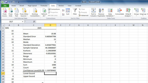
New data will appear on the spreadsheet and widen the margins to make it easier to see. At the bottom you will see the “Confidence Level” which we can use to work out the upper and lower bounds of the confidence interval. Type “Lower Bound” and “Upper Bound” in two separate rows beneath the table.

Step # 4 – Completing the Process
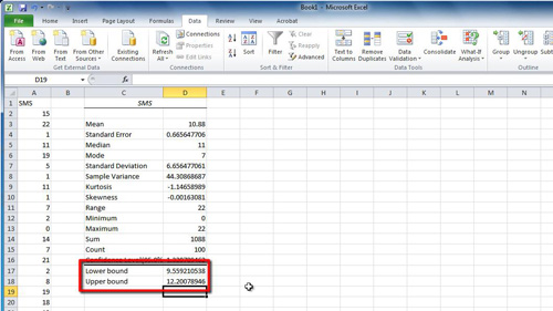
Next to “Lower Bound” enter an equation that subtracts the “Confidence Level” from the “Mean”. Next to “Upper Bound” enter an equation to add the “Mean” to the “Confidence Level”. The data indicates that we are 95% certain that the mean number of texts sent in a day by the class is between these two values and that is how to use excel confidence intervals.

 Home
Home