How to Sort Data in a Pivot Table or Pivot Chart

In this tutorial, you will learn how to sort data in a Pivot Table.
Sorting your data might be necessary when you are designing or examining a Pivot Table, in order to bring the values that matter first, or just to give it a sense of order.
Excel offers you some easy ways to do this.

Step 1.
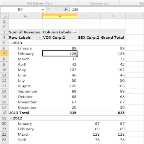
On the spreadsheet that we prepared, we put a sort function directly into the Pivot Table. This is standard for any new Pivot Table that is created. From here, we can choose to sort the columns alphabetically, in ascending or descending order.
open prepared Pivot Table

Step 2.
Apart from this option, you can select the Data menu on the ribbon and choose “Sort” on any of the fields in the Pivot Table: your data will update according to your selection.
choose Sort

Step 3.
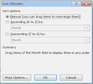
Click “Sort” from the Data menu on the ribbon and select “More Options”, then choose your primary sort key to sort by name of the month, and later on by year.
sort by more than one key

Step 4.
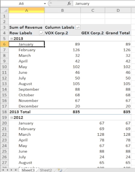
Click OK. The data will update according to your selection.
Excel displays the search results

Result: Congratulations, you have learned how to sort your data in a Pivot Table.

HowTech