In Google Docs, you can create and share your spreadsheets online. Tracking budgets and calculating values can be done very easily here. You can share your document with anyone and give them the right to edit the sheet. Insert charts and gadgets to express your data in the best manner possible. Use functions to calculate the values by using the specified cells automatically.
Follow this step by step Google Docs tutorial to learn how to work on excel file online in Google docs.
Step # 1 – Freeze the rows
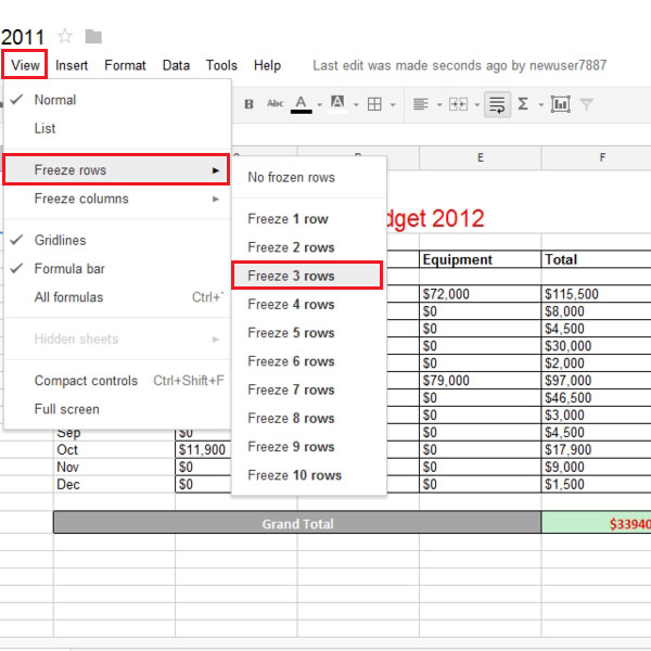
First of all, open the document that you want to work on. In this tutorial, we have selected a spreadsheet by the name of Budget. The freeze option allows you to freeze certain rows or columns. So when you will scroll down the spreadsheet, the headings above the frozen rows will remain fixed and appear all the time. When entering data, you will know exactly under which column you are entering it.
Step # 2 – Use the Average Function
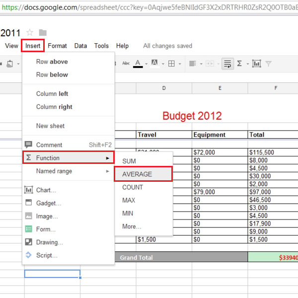
Google docs spreadsheet allows you to use some functions which can automatically calculate things instead of doing it manually. In this tutorial, if we want to calculate the average of “Training”, we can select that column and go to the insert tab. When the drop down menu appears, go to the “functions” option and select the “Average” function.
Step # 3 – Select the Cells
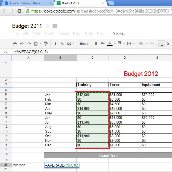
Customize the Average function by selecting the range for the formula by selecting the cells on which you want to apply the function. When the range has been set, click somewhere outside the formula or press the “enter” button. The average will be calculated. Another way of selecting the cells is by typing in the cell range manually. In the tutorial, we are concerned with the range from C5 to C16. So in the average function, we can write “C5:C16” in the range section of the formula.
Step # 4 – Insert a chart
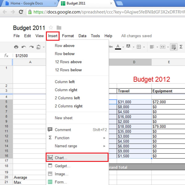
If you want to add a chart to your spreadsheet, first highlight or select the range on which you want to apply the chart. Once the range has been selected, click on the “insert” tab and select the “Chart” option.
Step # 5 – Customize the chart
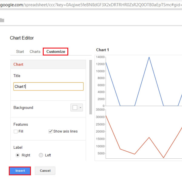
The “chart editor” will open in a new box. You can choose from a range of different charts. The Title, background features, labels and other settings can be selected and adjusted here. A preview of the chart will be showed to you in this box. When you are done, simply click on the “insert” button to add the chart to your spreadsheet.
 Home
Home