In a excel workbook when you enter numbers, all of them are formatted in a similar manner. You can choose to add different signs to them or even increase and decrease their decimal places etc. The date entries can also be formatted to show different formats in which the date can be displayed.
Follow this step by step tutorial in order to learn how to format dates in Excel along with numbers.
Step # 1 – Selecting the numbers
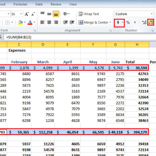
When you enter numbers in your excel workbook, you would surely know whether you are entering a currency or other values. In a case where you are entering values that signify expenses that were incurred on a monthly basis, you will need to display them in currencies. Thus, you will need to place a dollar sign in front of them. In order to do so, highlight the numbers you would like to format and then click on the “dollar” sign given in the “number” group within the “home” tab. Once this has been done, the selected cells will be formatted and will display a dollar sign. A comma sign will also be inserted.
Step # 2 – Decreasing the decimal places
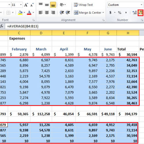
You can also change how many decimals you want to see. In order to do so, simply click on the “increase decimal” or “decrease decimal” button and make the desired changes. You might feel like the figures are being rounded off but actually only the decimal places will be hidden according to your changes. This makes it easier to read the values at a glance.
Step # 3 – Clicking on the Number group launcher
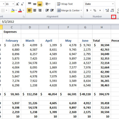
Moreover, you can choose to format the way the date appears in your worksheet. In this case, we have three different kinds of dates. The first one which says “created on” is just a number entry which is treated as text and the other two entries are functions. Select the first date cell and then click on the number group launcher.
Step # 4 – Selecting the date format
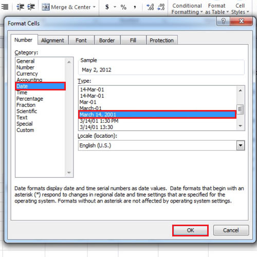
In order to practice how to format dates in Excel, from the dialogue box, select the style you want the date to be displayed in. There are a number of options that you can choose from. Scroll up or down in the “type” section under the “Date” tab and view the variety of styles available.
Step # 5 – Using the format painter
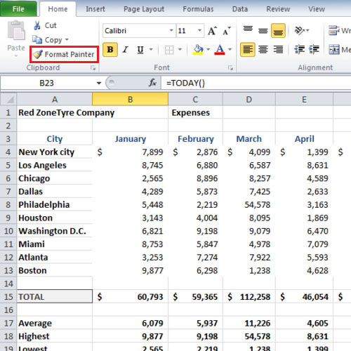
In order to format the other two dates, you can use the “format painter” feature. This feature allows you to copy the formatting of one cell and applying it to another.
First, select the cell from where you would like to copy the formatting and then click on the “format painter” option. Once this has been done, click on the cell you wish to apply the formatting to.
Step # 6 – Creating your own format
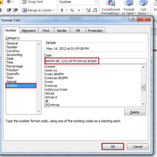
When we come to the last date entry, we notice that it displays the time as well as the date. In order to format this, select the last date entry cell and click on the number group launcher. While you are in the “custom” tab, edit the “type” bar to “mmmm dd, yyyy at hh:mm:ss AM/PM”. If you add the “Am and Pm” options, the date selected will be displayed in the twelve hour format.
Step # 7 – Clicking on the merge and center button
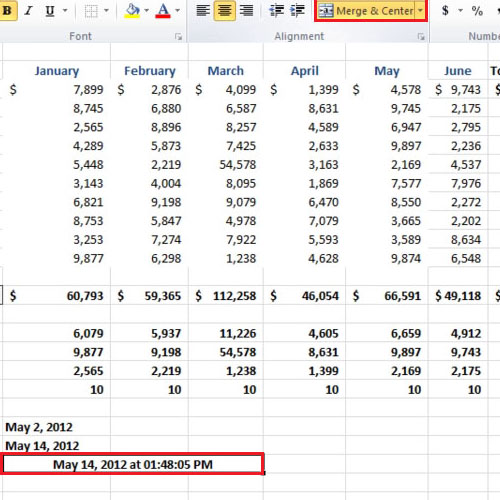
The format we have chosen makes the entry quite long and in order to make the cell bigger, you will need to merge the cells. Highlight the cells you would like to merge and click on the “merge and center” button given in the “alignment” group.
 Home
Home