While working with spreadsheets and workbooks in excel Microsoft, one can use a variety of fonts, background colors and borders to give their data a new and different appearance. You can even use the colors and borders for excel to make one cell stand out against the others or color code information.
Follow this step by step tutorial to learn how to apply fonts, background colors and borders in Excel.
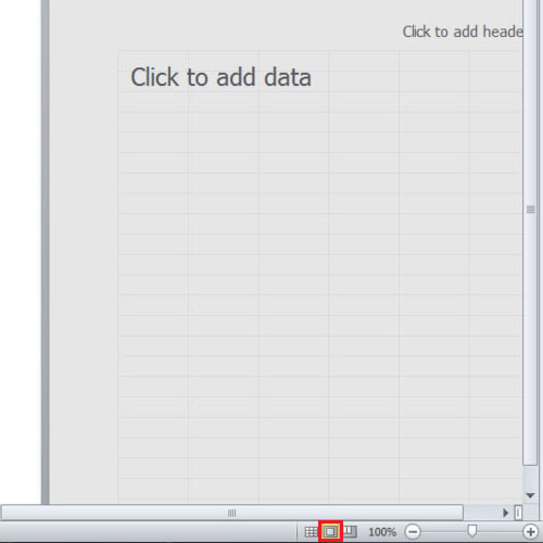
Step # 1 – Click on the “page layout” button
In excel Microsoft, we will look at the three kinds of views that you can use, by going to the lower right corner of the sheet. The middle button is for the “page layout” view. If you press this button, the page layout view will help you view how the sheet will appear when it is printed.
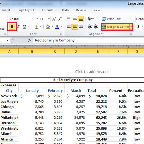
Step # 2 – Applying the merge and center feature
Working with headings can often be slightly tricky as one aims to make them stand out against the plain text placed in the worksheet. It is important to make sure the heading is placed in centre of the sheet. Now select all the cells from “A1” to “G1” and then press the “merge and center” button which is given in the “alignment” group under the “home” tab.
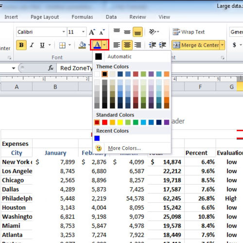
Step # 3 – Choosing the text color
Different colors can also be applied to the heading and in order to do so, click on the heading cell and then click on the text color button which is given in the “fonts” group. A drop down menu will appear in front of you displaying a variety of colors. Click on any one of them in order to apply it to the selected text.
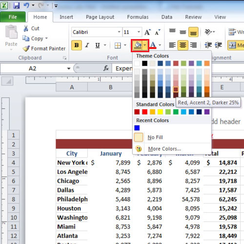
Step # 4 – Choosing the background color
In order to change the background color of the cell in which the heading is placed, click on the “fill color” button. From the “colors” drop down menu, click on any one color to apply it to the cell background.
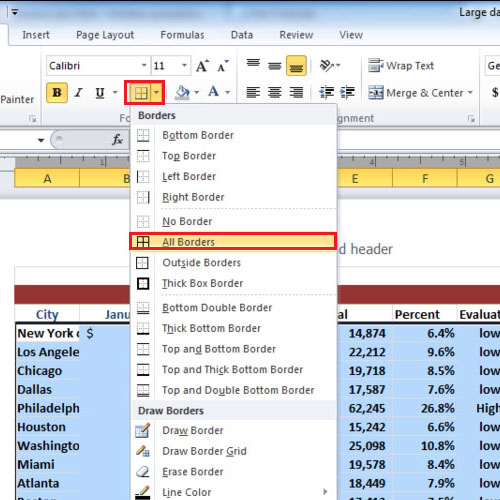
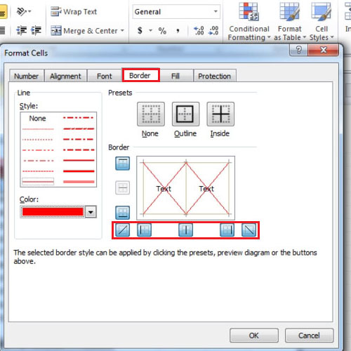
Step # 5 – Opening the border tab
When working with borders for excel and wanting to apply borders to the selected cells, right click on the chosen cell and then click on the “format cells” option. You can even do so by going to the “borders” button given in the “font” group. A dropdown menu will now appear from where you must select the “more borders” option. From the dialogue box that appears, go to the “border” tab and select the specific border you would like to apply to the cells.
Step # 6 – Applying borders to selected cells
If you highlight the cells and then click on the border button, borders will be applied to all the selected cells in one go. In this case, we have selected the “all borders” option to be applied to a certain range of cells.