In this excel tutorial, we will teach you how to apply conditional formatting in Excel. We will show you how to apply color scale. We will teach you how to insert highlight cells rule where cells get highlighted on a certain custom condition that you place. Furthermore, we will teach you how to make new rules in Excel. After creating these rules, we will show you how to manage them and use them to your advantage.
Step # 1 – Name the data range
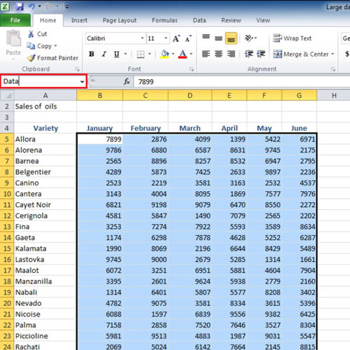
To start off the process, select the first cell of the data in your spreadsheet and press the “Ctrl + Shift + End” keys. The values will be selected. Now go to the “name” bar and type in the name of the range.
Step # 2 – Select a Color Scale
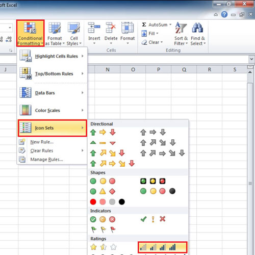
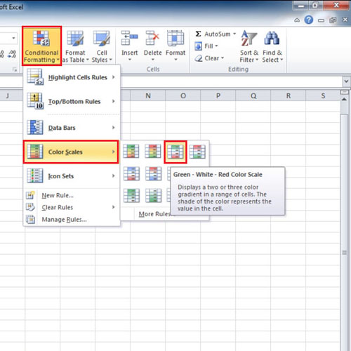
Once you have selected the data, click on the “conditional formatting” button under the “styles” group in the “home” tab. From the drop down menu that appears, select between “data bars”, “color scales” and “icon sets” here. Hover over the options given here and you will notice changes in your data. Click on any option and the relevant changes will be made to your data. Now go back to the “Conditional Formatting” button and select “color scales”.
Step # 3 – Apply the Highlight Cells Rule
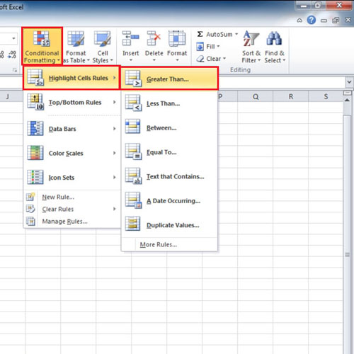
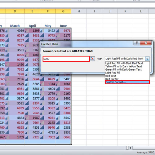
Here, you can apply the “highlight cells rules” option. Once you click on this, a number of options will appear. In this tutorial, we are selecting the “greater than” rule and putting in a conditional value. All values above this conditional value will be highlighted since the condition is of “greater than”.
Step # 4 – Change Background Color for highlighted cells
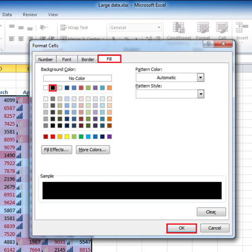
To change the way the values will be formatted, click on the “custom format” button and choose the text and the background color of your choice. Once this has been done, click on the “ok” option.
Step # 5 – Clear rules
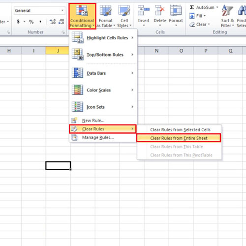
In order to remove the formatting, go back to the “conditional formatting” button and click on “clear rules”. Over here, select the “clear rules from entire sheet” option.
Step # 6 – Make a new rule
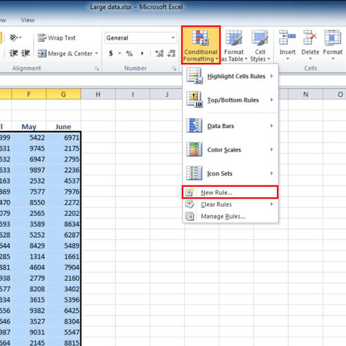
You can also make new rules by selecting the “new rule” option from the conditional formatting drop down menu. Once done, a new box will appear where you can select the rule type, format the style and perform other such actions.
Step # 7 – Set New Rule
Now, go to the “new rule button” and select the “format only cells that contain” option. Change the rule to “greater than or equal to” and enter the desired value. In this Excel tutorial, we are entering the value as “eight thousand”. Click on the “Format” button and change the font and the background color. Click on the “ok” button and preview the final output.
Step # 8 – Manage Rules
To change the rules again, go to the “Conditional Formatting” button and click on the “Manage Rules” option. A new box will appear allows you to edit, delete or add a new rule. This is how you will apply conditional formatting in Excel.
 Home
Home