You can hide a column and hide a row in Excel easily of you do not require that data for the time being. Such data can be removed from view and can be brought back anytime as per your requirement.
You can also group data in Microsoft Excel that allows you to manage it better.
To learn how to hide and group rows and columns in Excel, follow the tutorial below.
Step # 1 – Hide data
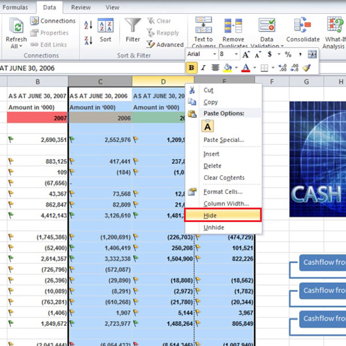
To hide rows or columns, select them, right click, and then click on the “hide” option. If you want to unhide them, simply drag your mouse across the hidden columns, right click on them and then select the “unhide” option. Over here we have dragged it across column “b to f”.
Step # 2 – Group the data
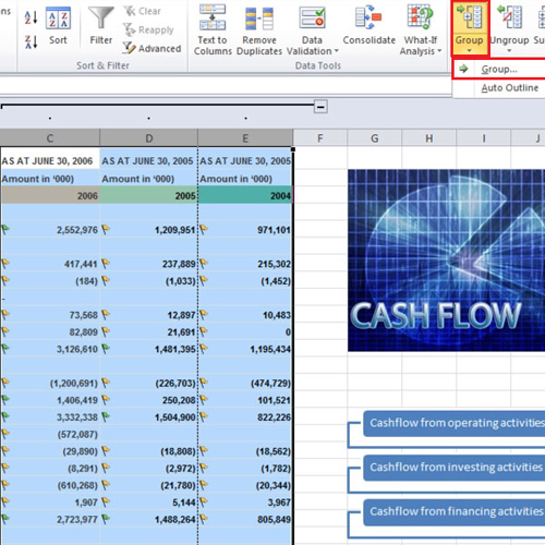
To group the column highlight it, go to the “data” tab, from the “outline” group select the “group” button and then select the “group” option.
At the top right you will notice that two buttons appear, “1” and “2” appear. If you click on them the groups will automatically “hide” or “unhide” depending on what you click.
Step # 3 – Group and hide rows
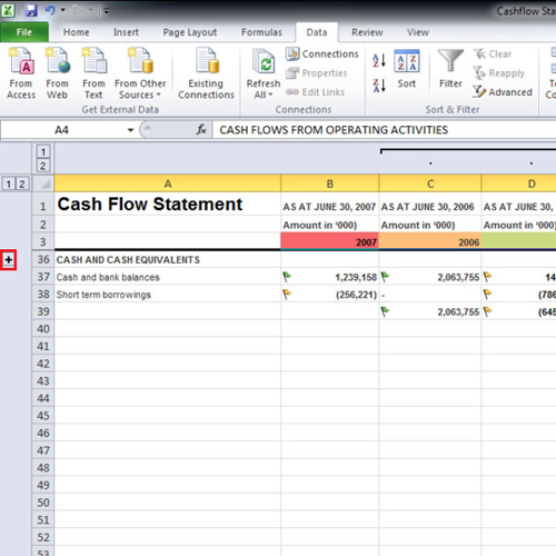
You can do the same thing to rows as well, highlight them, click on the “group” button and then select the “group” option. There will be a bar, you can either click on the buttons “1” and “2” that appear or click on the “plus and minus” buttons to hide or unhide data which are displayed along the rows.
Therefore, you can easily hide a row in Excel by using these buttons or the option you get from right clicking on the selected data.
Step # 4 – Go to “print preview”
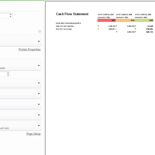
When you go to the “print preview” option you will see that if you have hidden something it will not be shown in the preview and therefore will not be printed.
Step # 5 – Ungroup data
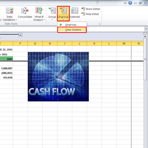
After you group data in Excel, you can easily remove these groups by clicking on the “ungroup” button and then selecting the “Clear outline” option.
 Home
Home