In this tutorial, we will teach you how to explore the analysis toolpak in Excel. First of all, we will show you how to enable Analysis toolpak. Once the toolpak has been enabled, we will show you how to work with it. Under data analysis, you will find several options. We will show you how to work with two of them in this video; correlation and moving average. We will show you how to apply both of the functions.
Step # 1 – Go to the Backstage View
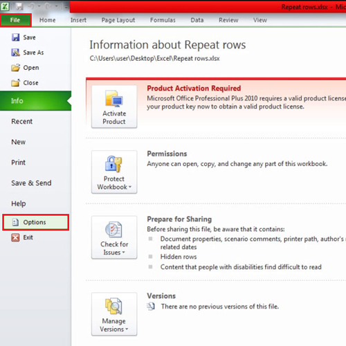
First of all you need to enable the analysis toolpak in Excel. Go to the “file” tab also known as the backstage view and click on “options”.
Step # 2 – Enable Analysis Toolpak
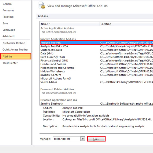
From the “excel options” window, go to the “add-ins” tab and select the “analysis toolpak” there. Click on the “go” button once you’re done. A small window will open up; select the first option which is the analysis toolpak and click on the “ok” button.
Step # 3 – Use the Data Analysis Option
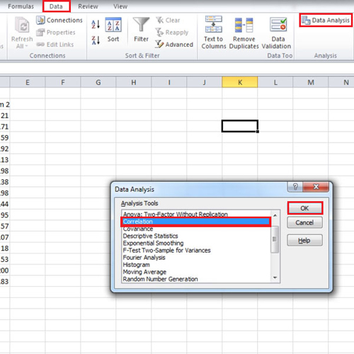
Analysis ToolPak has various options but we will work with only two in this tutorial. The first one is how to find correlation. Go to the “data” tab and click on the “data analysis” button on the extreme right. From the small box, select the “correlation” option and click the “ok” button.
Step # 4 – Apply Correlation in Excel
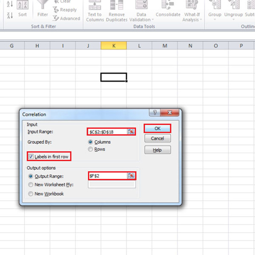
Now, the “correlation” box will appear on your screen. In the “input” range, select the cells which have data in them. If you include the first row which contains labels, then make sure the “labels in first row” box is checked. Lastly, select the “output” range. Click inside the box of the “output range” and then click on the cell where you want the output to be displayed. Click on the “ok” button to exit. The correlation result will be displayed to you.
Step # 5 – Apply Moving Average in Excel
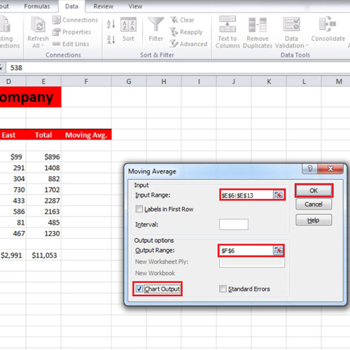
In the next sheet, we will take out the “moving average”. Click on the “data analysis” button and then select “moving average”. Click on the “ok” button and the “moving average” box will open up. Put in the range of input and since we are only going to select the “total” column without the labels so the “label” box should be unchecked.
Specify the cell where you want the output to be displayed in the output range. Before clicking on the “ok” button, check the box of “chart output”. Once done, the “moving average” will be displayed along with the chart.
 Home
Home