Many people don’t know how to create a PivotTable in Excel. They consider it too complicated. In the preparation of the Pivot table, you have to select the data range the Pivot Table is going to use. Next you choose the fields that you want to use in the Pivot Table. Then you assign these fields roles; place some in rows while others in column headings. In this tutorial, we will teach you how to create a basic Pivot Table in Excel.
Step # 1 – Insert Pivot Table
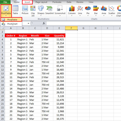
First of all, go to the “insert” tab and click on the “pivot table” button which is located in the “tables” group. From the drop down menu, select the “pivot table” option.

Step # 2 – Select data for Pivot Table
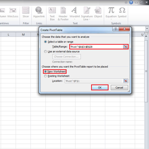
Once done, the “pivot table” box will open up. Select the range of the data including the top row and then click on the “new worksheet” radio button before clicking on the “ok” button.

Step # 3 – Configure Pivot Table
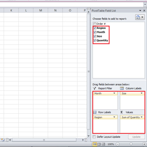
A new sheet will be added to the workbook but the data will not be lost. On the right hand side of the screen, you will find the “pivot table field list” pane. The fields will be listed in the box. In this tutorial, we clicked on the “region” field and dragged it to the “row labels”. Next, drag the “size” field to the “column labels”, the “sum of Quantity” field to the “Values” and the “month” field to the “report filter”.

Step # 4 – Results of the Pivot Table
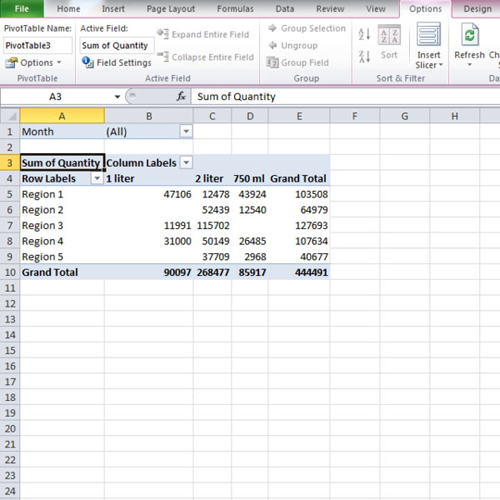
Now as you can see that in the “row labels”, we have the “regions” from one to five. Then in the “column labels”, we have the size. We have grant total region wise as well as size wise in the Pivot Table.

 Home
Home