For the purpose of this tutorial, we will be working with a pivot table. We will apply multiple filters to it in order to filter the data. Furthermore, we will teach you how to apply the slicer option in Excel. Slicer is a quick way to find out the relevant data if you are using one filter at a time. And lastly, we will teach you how to modify a PivotTable in Excel.
Step # 1 – Filter Pivot Table
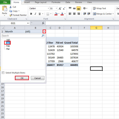
When you have a pivot table, you can filter the data by simply clicking on the downward pointing arrow and selecting the sort criteria. In this video, we have selected the month of January.
Step # 2 – Apply multiple filters
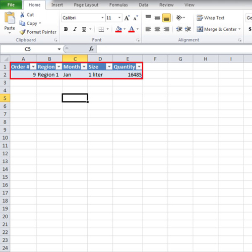
Consider there might be a scheme on “1 liter” bottles in “region 1” in the month of January and we want to know the specific data.
Thus, with the month of January, we just wanted the data for 1 liter bottles. Lastly, we further narrowed our filter criteria and selected “region 1” only.
Step # 3 – Clear Filters
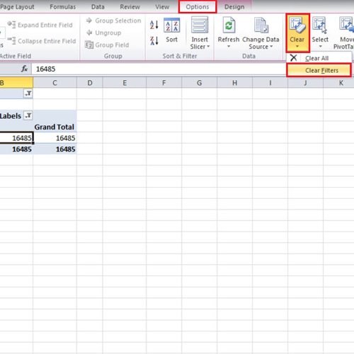
If you double click on any data, it will show you all the relevant information about it. If you want to remove your filter, go back to the “options” tab and select “clear filters” option from the “Clear” drop down button.
Step # 4 – Modify pivot table
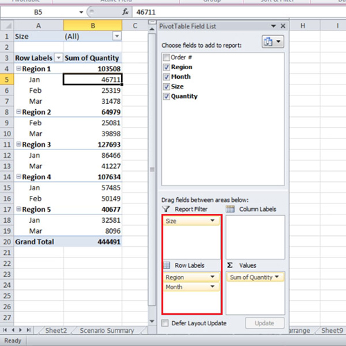
Now we will show you how to modify a pivot table in Excel. Click on “month” and drag it to the “row labels” and place it below “region”. Now the months will be separated by region.
If you drag “size” to “report filter”, then you can filter it by size as well. Let’s suppose, we want to see only the data of “2 liter” bottles so click on the downward pointing arrow of “size” and select “2 liter”.
Step # 5 – Apply Slicer option
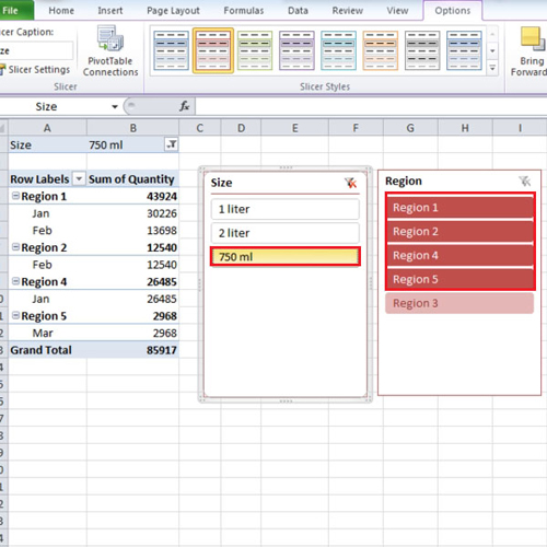
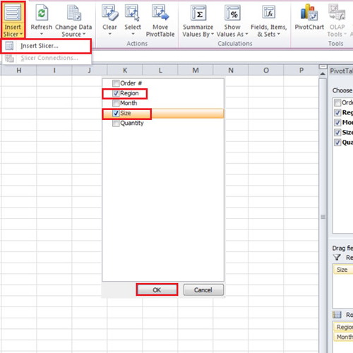
In the pivot table, “Slicer” can be inserted as well. Go to the “options” tab and click on the “insert slicer button”. From the “insert slicer” box, select the fields by which you want to filter. You can change the colors of slicer through the “options” tab.
Step # 6 – Functionality of Slicer
In this tutorial, when we click on the “750 ml” button from the “size” slicer, automatically the data changes in the “region” slicer accordingly. So, we know the regions where the 750 ml bottle is present. Therefore slicer helps you if you want to find the data quickly by choosing one filter at a time.