In this tutorial, we will teach you how to insert Spark lines in Excel. Sparklines in Excel help you express your data graphically. There are several types of sparklines such as lines, columns or win/loss. In lines, you can view the ups and downs, the peaks and slumps while in win/loss the negative points will be shown in a different color. We will also show you how to change the styles on these sparklines.
Step # 1 – Insert Sparklines
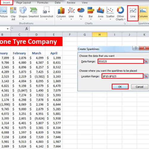
Go to the insert tab and from the “sparklines” group, click on the “line” button. A small box will appear; select the “data range” and then select the column for the “location range” where the sparklines will appear.
You can easily increase the size of the lines by stretching your column width.
Step # 2 – Change Marker Color
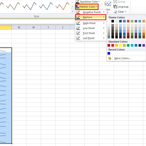
From the “design” tab, click on the “marker color” button and go to “markers” and from there choose a color for the markers. All the points will be highlighted.
Step # 3 – Display High & Low Points
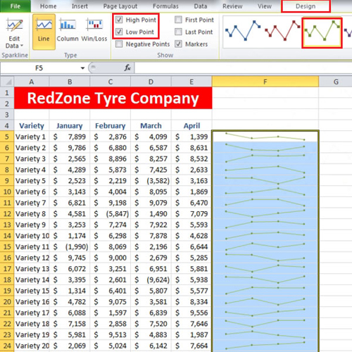
If you want to see the high and low points, you can check their respective boxes which are located in the “show” group. Next, you can choose the “style” of the lines. Click on the downward arrow and from the various options that appear in front of you, choose any one of them. Likewise, if you want to see the negative points, tick its respective checkbox.
Step # 4 – Apply Win/Loss Structure
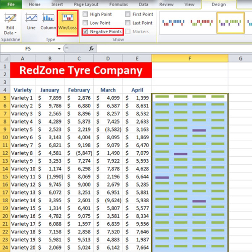
From the “type” group, you can change the type of sparklines. Click on the “Win/Loss” button and it will show you bars with the negative points highlighted in another color.
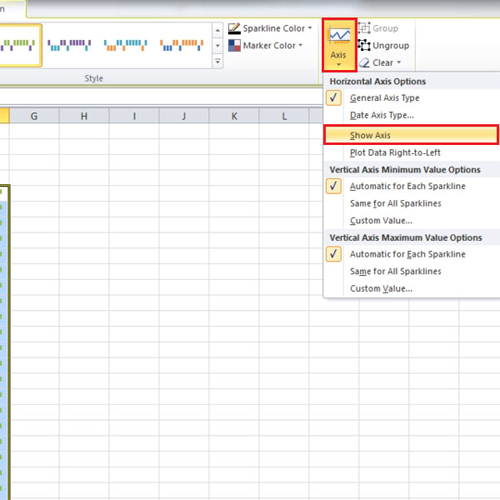
Step # 5 – Show Axis
If you want to see the axis, click on the “axis” button and select the “show axis” option.
 Home
Home