Microsoft Excel is a program which specifically allows you to use spreadsheets in order to organize your data and perform complex mathematical calculations. When working with these Excel sheets, one can perform various activities with the cells in order to make them stand out or even apply color to them. Apply styles to your worksheet and give it some final touches. This allows the user to customize the sheet and give it a personalized touch. There are a variety of styles already provided by the program, but one can moreover, even create their own customized styles, as per their requirements.
In this tutorial we will teach you how to apply, create and share styles in Excel.
Step 1: Selecting a style
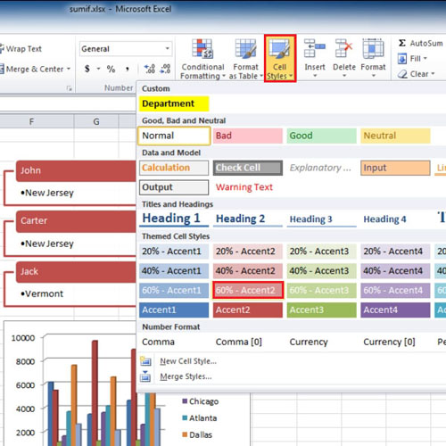
When working on an excel sheet, you might want to color code specific cells or apply styles to them in order to make them stand out amongst the rest. In order to do so, highlight the desired cells and click on the “Cell Styles” button in the “styles” group. From the drop down menu, select a style and while moving the cursor over different styles, you will notice the highlighted cells will change.
Step 2: Applying styles to numbers
One can even apply cell styles to numbers in the spreadsheet by clicking on the “Cell Styles” button again and then selecting the “Currency[0]” option. The numbers will now start displaying a dollar sign before them.
Step 3: Naming the style
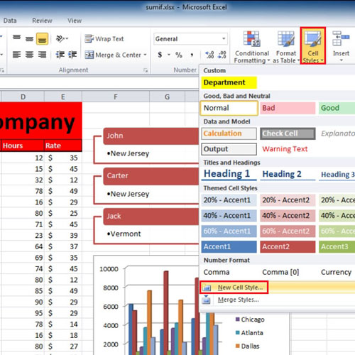
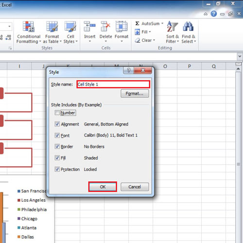
Now highlight a few new cells as per your requirement and go to the “Cell Styles” button. Click on the “New cell styles” option and a dialogue box will appear on your screen. You can give this style a certain name and click on the “ok” button in order to proceed further.
Step 4: Applying a custom style
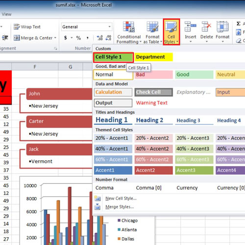
In case you want to apply the custom style you just created to some more cells, highlight the desired cells and go to the “Cell Styles” option. Once you are done, click on the name of the style you wish to apply and changes will automatically be made to your Excel sheet.
Step 5: Modifying styles
You might even realize you want to modify some styles. In this case, right click on the style you would like to make changes to and select the “modify” option.
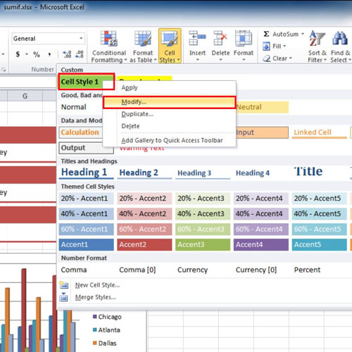
Step 6: Formatting styles
Once the above steps have been completed, click on the “format” button and make the desired changes. Now click on the “ok” button after which you will notice the changes will take place.
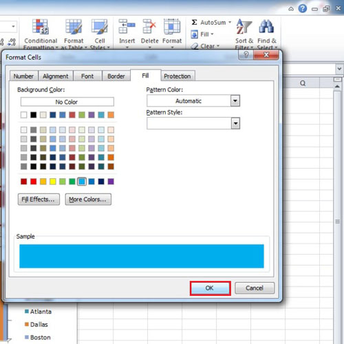
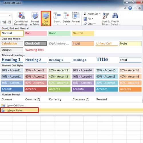
Step 7: Merging Styles
You can also choose to use the custom style that you created in another work book. In order to do so, open the original file and the new workbook simultaneously and highlight the desired cells. Now go to the “Cell styles” button and then click on the “Merge styles” option.
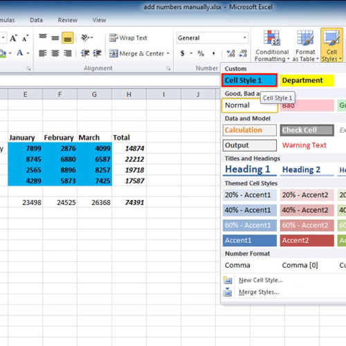
Step 8: Applying the custom style
Over here, select some styles and go to the “cell styles” button. Next, select the custom style after which changes will be made to the cells in your spreadsheet.
 Home
Home