MS Excel provides its users with the option of using a variety of features to make their worksheets stand out, and make them appear more attractive. It allows them to add graphics, pictures and shapes in Excel worksheets. One can also add a number of effects to their pictures, change its shape, or add colors to them.
Follow this step by step tutorial to learn how to use excel add ins while working with Microsoft Excel.
Step # 1 – Adding a picture
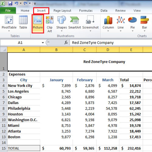
First of all, in the excel worksheets go to the “insert” tab and click on “picture” button. A drop down menu will appear from where you can browse through a variety of pictures and select one that you would like to use in your sheet. Once the picture has been inserted, click on the “handles” which appear when you click on the picture and drag them to adjust the size of the picture as per your requirements.
Step # 2 – Choosing the “set transparent color” option
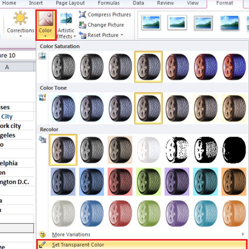
When any picture is inserted in a worksheet, it covers the background since it has a white border. You can change this by clicking on the “color” button and select the “set transparent color” option from the drop down menu. Now click on the border of the image. You will notice that now the background on which the picture was placed will be clearly visible.
Step # 3 – Setting the picture color
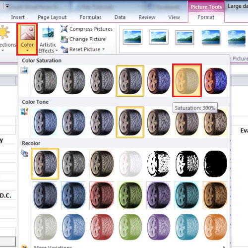
In order to alter the color saturation, tone and recolor the image, go to the “color” option. Other effects can also be applied to the picture by clicking on the “artistic effect” button. In this tutorial, we have changed the color saturation of the picture and given an artistic effect to it in order to give it a complete look.
Step # 4 – Adding a clip art
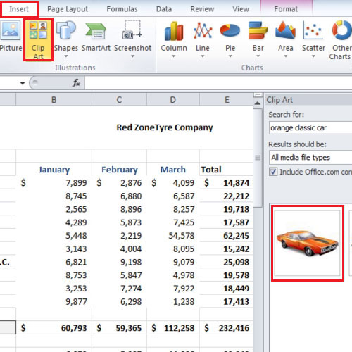
When you want to insert a clip art in a worksheet, you can use excel add ins. Click on the “insert” tab and then click on the “Clip art” button. On the right hand side, you will notice a bar appear. You can select a clipart from here by double clicking on it, after which it will automatically be inserted into the worksheet. You can now drag the clipart to any part of your worksheet, depending on where you would like to place it.
Step # 5 – Selecting the “Clear all” button
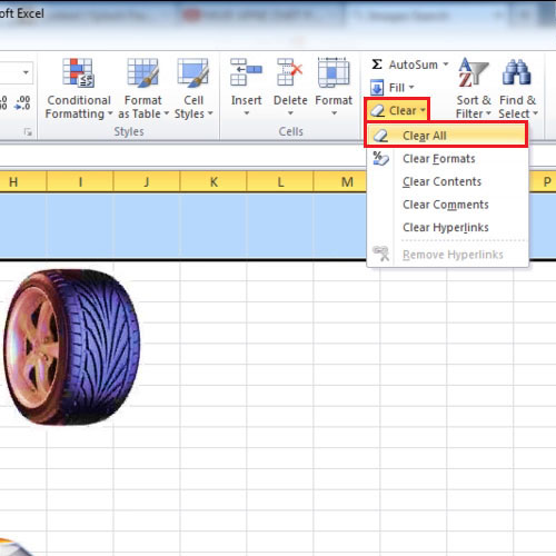
In order to add shapes to your worksheet, you firstly need to go to the “insert” tab. However, before doing so, make sure the cells where you want to add the shape are clear of all data. In this case, the first row in the sheet contains some text which must be cleared before the shape is inserted. In order to clear this data, select the specific row or column and go to the “home” tab. Now, from the “editing” group, select the “clear” button.
Step # 6 – Inserting a shape
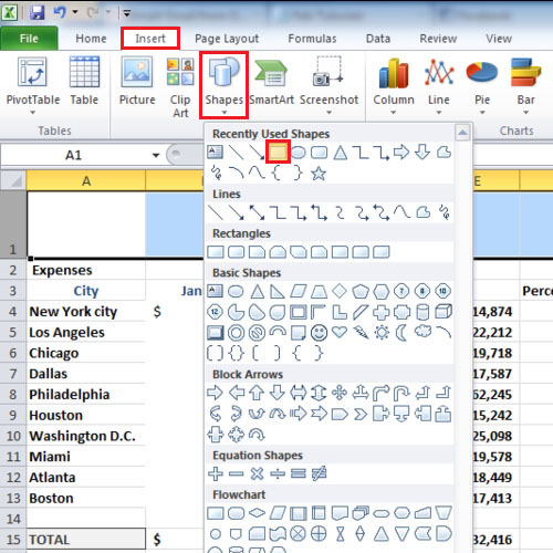
Once the above steps have been completed, go to the” insert” tab and click on the “shapes” button. Select the type of shape you would like to insert and then press the “alt” key. You must now drag the mouse pointer and then release it in order to fill the desired row.
Step # 7 – Changing the theme of the shape
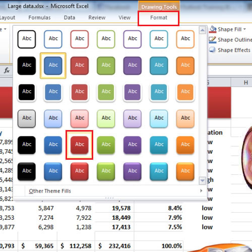
You can also choose to change the color of the shape. In order to do so, click on the downward arrow given under the shape styles and choose the color. Now, add some text in the shape and change the font color or font size as per your requirements from the “home” tab.
Step # 8 – Using the “more gradients” button
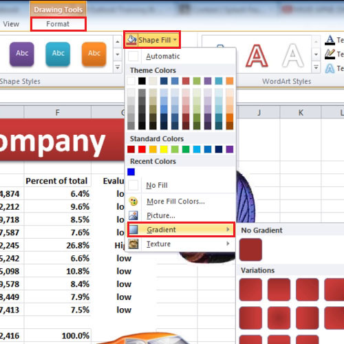
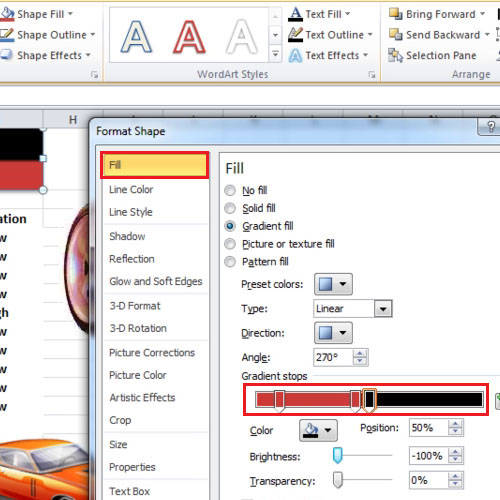
Moreover, go to the “format” tab and click on the “shape fill” button. From the drop down menu, select the “gradient” option after which a list will appear in front of you. From here, click on the “more gradient” option in order to proceed further.
Step # 9 – Going to the fill tab
A “format shape” box will now open. Using this, you can change the “brightness, transparency, color” etc as per your requirements. In this case, we are changing the position of the “gradient stops”. You will be required to click on the three different stops and drag them to change the appearance of your shape.
 Home
Home