In this video tutorial we will show you how to make excel gantt chart.
In order to create gantt chart in excel, open your document. Select your data in the excel document. Go to the “insert” tab. Click on “Bar” and select “2-D Bar”.
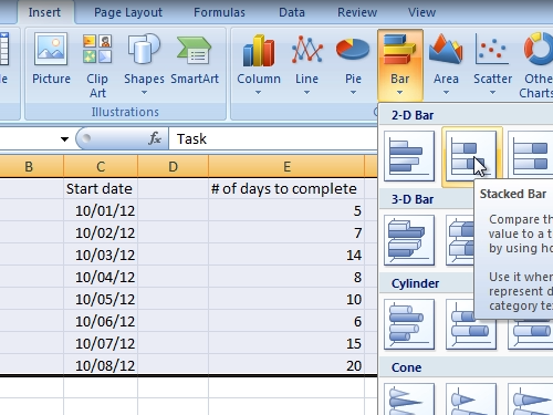
Adjust the position and size of your chart. Right-click on “C2” cell and choose “Format cells”.
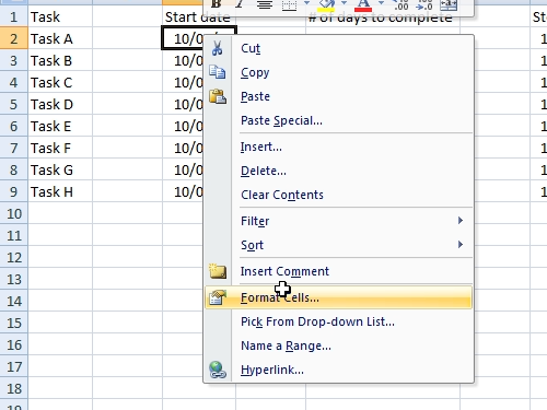
In the appeared window, go to “number” tab and choose “general” category. Then go to your “G9” cell, right-click on it and choose “Format cells”. In the appeared window, go to the “number” tab and choose “general” category. Now select the data under the chart, right-click and choose “Format Axis”.
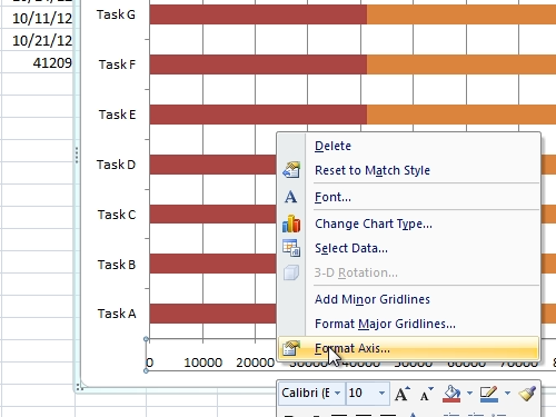
Select “fixed” to minimum and set the value to your C2 cell, in our example “41183”. Also, select “fixed” to maximum and set the value to your G9 cell, in our example “41209”. Change the “Major unit” to “Fixed” and set the value to “1”. Then set the “Axis value” to “41183” in “vertical axis crosses” and press “ok”. Now go to your “G9” cell and set “date” category in the “number” tab. Then change your data in “C2” cell the same way. Now select the data under the chart, right-click and choose “Format Axis”. Go to the “Alignment” tab and set “custom angle” value to “-45”. Then, go to the “Number” tab and set “date” category. Close the window. Right-click on left axis title and choose “Format axis”. In the appeared window, check “categories in reverse order” in the “axis options” tab. Also set “horizontal axis crosses” to “At maximum category”.
Now, select a part of a column chart by clicking a mouse on it. Then, right-click on it and choose “Format Data Series”. In the opened window go to the “Fill” tab and select “no fill”.
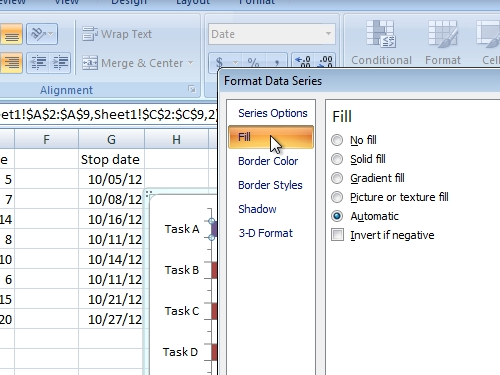
Then go to the “Border color” tab and set “no line”.
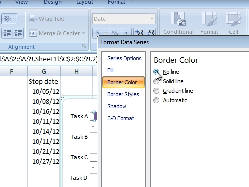
Select another part of a column chart by clicking on it. Right-click on it and choose “Format Data Series”.
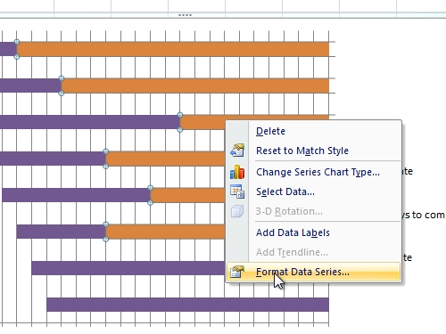
In the opened window, go to the “Fill” tab and select “no fill”. Then go to the “Border color” tab and set “no line”. You can also adjust text size.
Now all you have to do is to remove legend text, except the column part that left. Right-click on your chart and choose “move chart”.
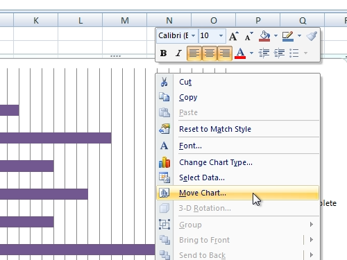
In the move chart window select “new sheet” and name it “Gantt chart”. Now your gantt chart is ready.
 Home
Home