While working with spreadsheets in Ms Excel, using a variety of shortcuts and cell references can save you a lot of time. You can name cell ranges and use that name later on instead of typing out the range over and over again. Moreover, the cell names can also be used while entering a function or formula.
Follow this step by step Ms Excel tutorial to learn How to Name and use cell ranges in Excel.
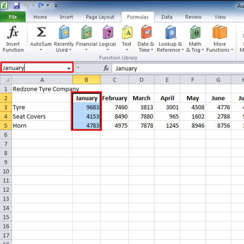
Step # 1 – Entering the range name
In this Ms Excel tutorial, we will start off the process by giving the cell range a name. In order to do so, highlight the cells that you want to name and go to the name box which is situated on the left side of the screen. In this case, we have highlighted the data of January and in the name box written “January”. When you will click on the name drop down menu, the name of the range will appear and when you will click on the name, the data range will be selected automatically.
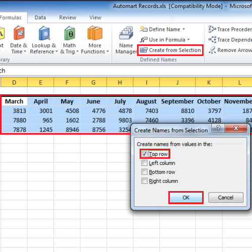
Step # 2 – Click on the “Create from selection” button
An easier method of doing the same thing is to highlight the entire area and go to the “formulas” tab. In the “defined names” group, click on the “create from selection” button. Once this has been done, a small box will appear. Over here, select the top most option and click on the “ok” button.
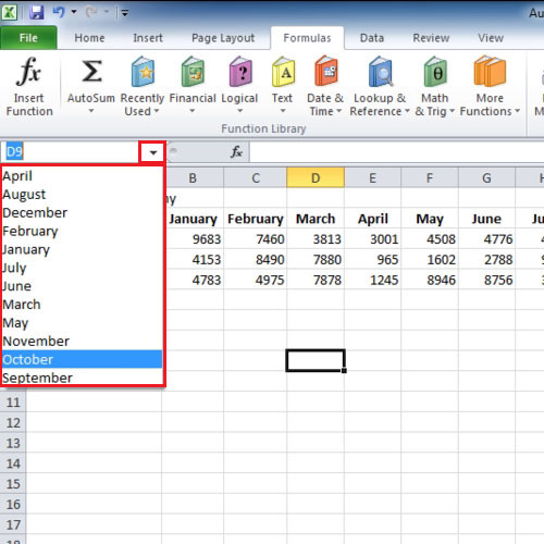
Step # 3 – Viewing the range names
Once you use the “create from selection” option, all the titles of the columns will be taken as the names. Now in the name box, you will see that all the names of the months be given as headings.
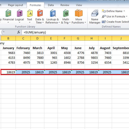
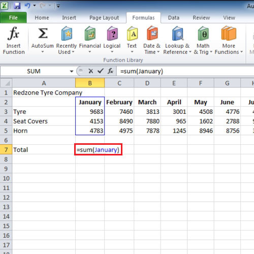
Step # 4 – Entering the range name in the function
The names of cell ranges can be used in functions as well and instead of entering range, you can type out the name of the range. In this case, suppose we want to use the “sum” function to calculate the total for each month. While entering the sum function to calculate the total for the month of January, we will write “January” within the brackets which will automatically define the range.
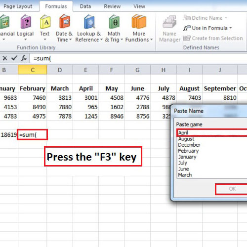
Step # 5 – Pressing the F3 key
When inserting formulae, you can use the shortcut of pressing the “F3” key; it will show you all the names that you have stored to be displayed in “paste name” box.
Step # 6 – Using the “Autofill” handle
However, the downside of using this method is that if you try to use the “autofill” option, it will not work. Instead, it will only copy the sequence of the highlighted cells that you have selected in order to use the autofill feature.