Macros are scripts that you record; certain actions you may perform in a specific sequence. You might have to perform a set of actions in a particular order on a day to day basis. Instead of doing it manually, do it just once when recording the macro. Next time you want to perform those set of actions, simply run the macro.
In this tutorial, we will teach you how to record and use a simple macro in Excel.
Step # 1 – Add Developer tab
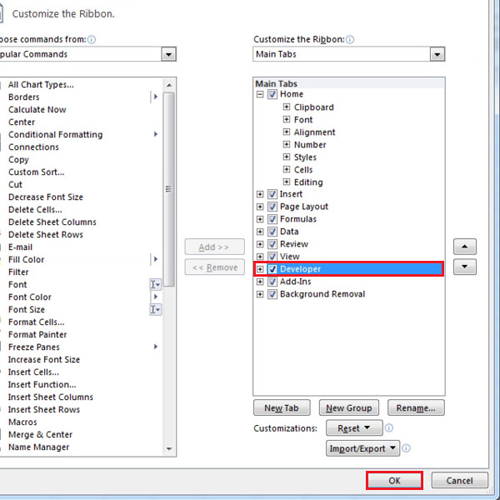
First of all, you will be required to add the developer tab. In order to do that, go to the back stage view and click on “options” button. From the “excel options” window, click on “customize ribbon” tab and then check the “developer” option.
Step # 2 – Record Macro
Now return back to your sheet and open the file from which you want to get the data. Press “ctrl + F6” to switch between workbooks and return to your original workbook.
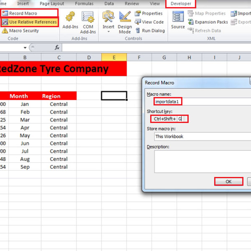
Click on the “developer” tab and from the “code” group, click on the “use relative reference” button. Then click on the “record macro” button.
You can name your macro in Excel but make sure that there are no spaces between words. Next, select the shortcut key. In the video, we have used “shift” and “g”, so the shortcut key would be “ctrl + shift + g”. You can add description of your macro if you want to. Press the “ok” button and your macro will start to record. Since we are using relative references thus we have make sure that the keys we press will not leave any cells and the data gets pasted to the first empty row it finds.
Step # 3 – Perform actions you want to record in the macro
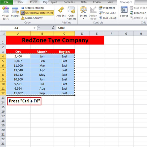
In the tutorial, we pressed “ctrl + home” and then “ctrl + down arrow”. Again press the “ctrl + down arrow” and you will reach the last cell that has data in it. Press the “down arrow” once more to go to the empty row and then use the short cut key to switch between workbooks. Press “ctrl + home” and then press “ctrl + down arrow” and it will take you to the “column header”. Since we do not want to include the column header twice, we pressed the “down arrow” and went to the first cell that has data in it. Using your mouse will not help in selecting the data because we want to automatically cover all the data regardless of how may rows or columns it has. In order to do so, press “ctrl + shift + down arrow” and then press “ctrl + shift + right arrow”. After the entire data is selected, copy the data and switch back to the original workbook by pressing “Ctrl+F6”.
Step # 4 – Stop Recording the Macro
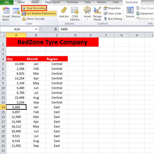
Paste the entire data you have selected and click on the “stop recording” button to stop. Use the escape key to remove the copied data from the clipboard. This is how you record macros in Excel.
Step # 5 – Run the recorded Macro
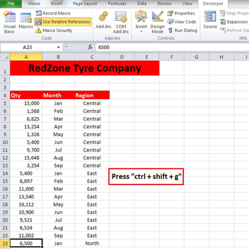
Now close the other workbook and open a new one from which you want to get the data. When the new workbook opens, use “ctrl + f6” to switch back to the original workbook. Press “ctrl + shift + g” which is the shortcut you assigned to run the macro and the data will be copied and pasted automatically.
Use this as many times as you like with as many workbooks you want to. This is how you make use of the recorded macros in Excel.
 Home
Home