In this tutorial, we will teach you how to work with excel VLOOKUP function. In Excel, VLOOKUP functions are used to find specific information in large data tables. As the name suggests, vertical lookup looks for a value in a table which has data entered in columnar format.
Step 1 – Enter the data
Follow this step by step guide to learn how to work with excel VLOOKUP function.
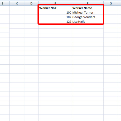
First of all, open a workbook in Excel and make two sheets. Enter the data on one sheet while the VLOOKUP formula on the other sheet. For the purpose of this tutorial, we will insert the worker number and the VLOOKUP formula will give us the worker name. The data containing the names and the numbers of the workers is written on sheet 2.

Step 2 – Enter the VLOOKUP function
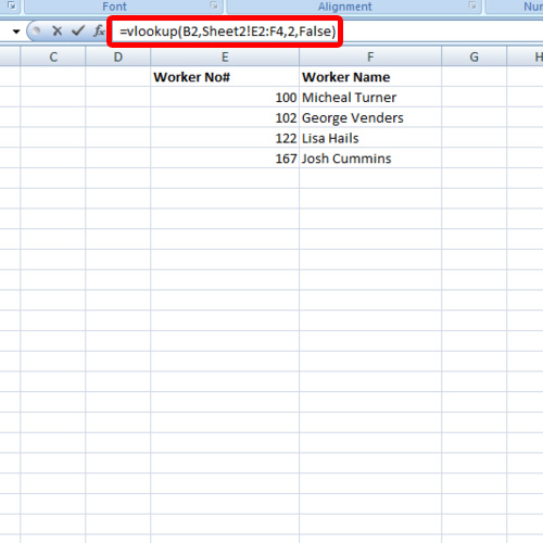
In the cell next to the worker name field, type in the following:
=vlookup(B2,Sheet2! E2:F4,2,false)
In Excel, VLOOKUP functions require you to enter the lookup value, the table array, the column index number and true or false condition at the end of the function.
In the formula, B2 refers to the lookup value. The table array or the data range we are dealing with is on sheet 2 and in the cells E2:F4. The names of the workers are written in the 2nd column of the table thus the number 2 for column index number. At the very end, false was inserted because we wanted an exact match.

Step 3 – Check if the formula works
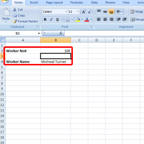
Let us try if the formula actually works. We will insert a worker number that is mentioned in the data written in the other sheet. The respective worker name for the number will be displayed in the cell where the formula was inserted. If you will insert a number which isn’t available in the data range forming the part of your table array, an error will be displayed.
In this manner, you can apply the VLOOKUP function and work with multiple sheets.

 Home
Home