This tutorial will talk about and explain a few keyboard shortcuts in Excel that allow you to work more efficiently in this software.
Knowing different shortcuts in Excel gives you the opportunity to save time by working faster and more accurately while using this program.
To learn more about these shortcuts, follow the tutorial given below.
Step # 1 – Press the “ctrl + end” command
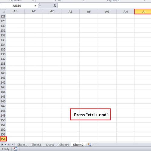
When you press the “ctrl + end” key, you will be taken to the last row and the last column which was used by you. In the video, column “Ai” and row “36” represents the last cell. Usually what happens is we sometimes copy something in the sheet and use it as a rough work area. We delete it later on but Excel remembers the range of the sheet that you have been to.
In our case, it was row “36”. In the video, we will go to row “154”, type in something and then delete it. Now when you go to the top and press the “ctrl + end” command, it will take you to row “154” and column “AI”.
Step # 2 – Use the “ctrl + a” command
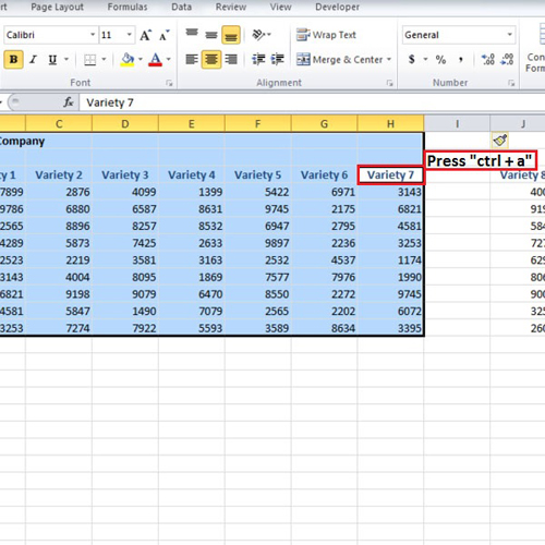
An issue regarding selection is related to the continuity of the data. This means that if you press “ctrl + a” in order to select all the data while being in a cell which has data in it, it will only select the cells up to the area where there is continuity. However, if you click on any empty cell and press “ctrl + a” there, the whole sheet gets selected.
Step # 3 – Select data in an entire column
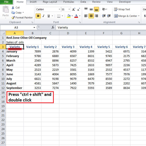
An easy way of selecting the data in an entire column is that when you select a cell, a box appears around it. Double click on the bottom line of the box while pressing the “shift” and the “control” key. If you press only the “control” key then you will be taken to the last cell which has data but it will not get selected. You can select entire rows using the same trick but to do that you will have to double click on the right side of the box.
If there are any hidden rows or columns, click on the top left button which selects the entire sheet and then double click on the divider of the rows or columns. After doing so, the hidden rows or columns will be displayed.
Step # 4 – Copy data without the hidden rows
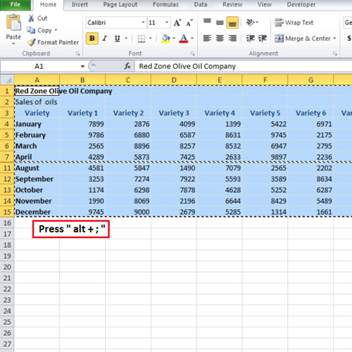
Let’s suppose we do not want to copy certain rows. Simply select them, right click on them and choose the “hide” option. Now copy all the data and paste it in a new sheet. Notice that although the rows were hidden when we copied the data, still they got copied. You can avoid this from happening. Along with other shortcuts in Excel this software also provides you with a shortcut for copying data without the hidden rows. To do this, when you select your data press “alt + semicolon” and only the visible data will be selected. The lines will show you the start and the end point of the hidden data.
Step # 5 – Click on the “find and select” button
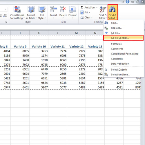
Another way of selecting the visible data is by going to the “find and select” button and from the drop down menu, selecting the “go to special” option.
Step # 6 – Select the “visible cells only” option
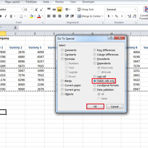
When the box appears, click on the radio button of “visible cells only” and then click on the “ok” button.
The different keyboard shortcuts in Excel explained in the tutorial above will help you while you are working in this software by Microsoft Office.
 Home
Home