In this tutorial, you will learn about the status bar in Excel and how it is useful to the user. This feature of Ms Office Excel allows you to view different totals like the average, sum, etc by simply selecting the cell whose values you want to figure out.
You can even customize the status bar so that it shows the mathematical values that you need rather than the ones present there by default.
To learn how to customize the status in Excel, follow the tutorial below.
Step # 1 – View the status bar
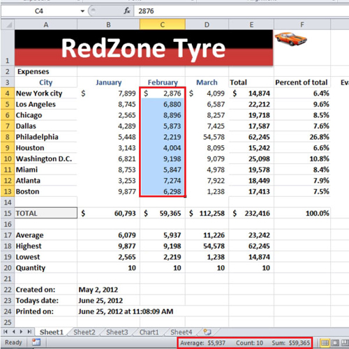
Sometimes you only want to see the total of something for a while and do not want to include a whole column while doing so. Status bar helps you do this; when you select more than two cells which have values in them, you can see the total sum of those cells along with their average in the status bar.

Step # 2 – Select two cells horizontally
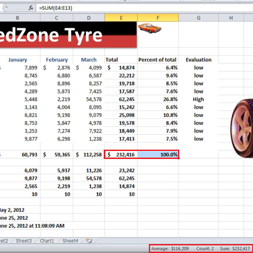
It does not matter whether you drag and select your cells horizontally or vertically; their sum, count and average will be calculated. Minimum of two cells are required to be selected for the calculation.

Step # 3 – Customize status bar
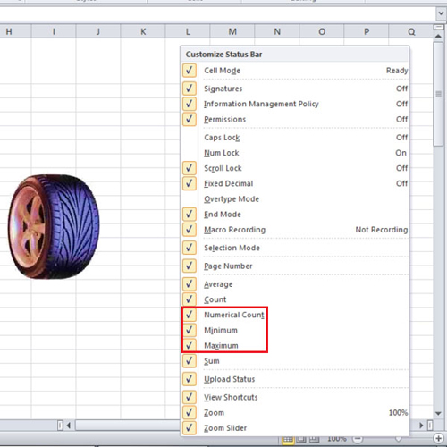
Now let’s go and customize the status bar. Right click on the status bar in Ms Office Excel and you will see a list of options, most of them will be ticked already. Tick the three options by the name of, “maximum, minimum and numerical count”.
When you will select the cells now, not only the sum, count and average will be calculated but also the numerical count along with the minimum and maximum values will be shown.

Step # 4 – View the customized status bar
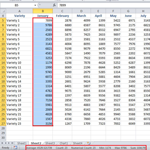
In the video when we go to “sheet 2” and select column “b”, you will see that it has twenty three values and the lowest number is one “1174” while the maximum is “9786”.
It is really helpful if you want to take a quick look at the quarter sales; select the three cells and it will show you the sum of the three months.
You can make good use of the status bar in Excel as it will help you by easily providing you with values that you require.

 Home
Home