In this tutorial, we will show you how to use time with currency calculations in Excel. There are several times when you have time and currency calculations. For example, we have the number of hours that a person has worked and the hourly wage rate. We have to calculate the total wage. Both the things have different units thus cannot be computed by doing simple multiplication. We will show you how to perform in such calculations.
Step # 1 – Insert multiplication formula
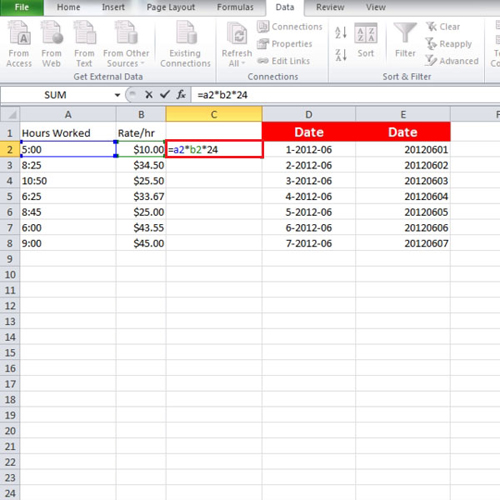
In this Ms Excel tutorial, you will notice we have a column which contains the number of hours that a person has worked and in the column next to it, we have the hourly wage rate.
To calculate the total wage, write
“= a2*b2*24”
So we will get our answer using this formula. And we can fill in the rest of the column by using the “auto fill” function.

Step # 2 – Convert Text to Columns Wizard
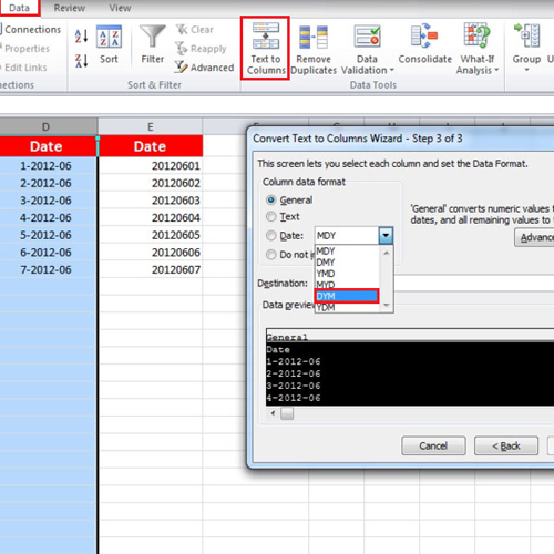
Now in order to format a date, highlight the cells or simply highlight the entire column. Once done, go to the “data” tab and click on the “text to column” button located in the “data tools” group.
A box will open and on the top it will be written “Step 1 of 3”. We have to skip to step three so click on the “next” button until you’re on step three.
When you are there, click on the drop down menu and select the order in which you want your date to be written. In the tutorial, we selected “dym” and clicked on the “finish” button.

Step # 3 – Change to YMD format
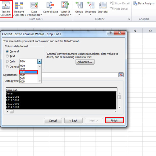
The next column of date has year at the beginning, then the month and then the day. So this will be formatted in the same way by going to the “text to column” button. In the third step, click on “ymd” and then click on the “finish” button in MS Excel.
Doing so will result in the date to be written as year first, month second and day in the very end.

 Home
Home