Microsoft Excel allows you to work on a spreadsheet which can be used to organize information. One can even carry out calculations while working with excel column numbers using a number of formulae and functions given. In this tutorial, we will show you how to use some of the basic functions while working with numbers present in the columns. We will help you better organize your data in column format.
Follow this step by step tutorial in order to learn how to use Microsoft excel while working with numbers in columns.
Step # 1 – Calculating the Average
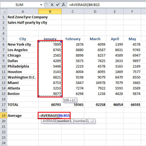
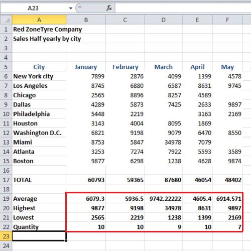
In order to calculate the average sales for the month of January, click on the cell under the “total” heading and type “average”. Now click on the cell and type “=Average(B6:B15)” and press the “Enter” key once you are done; the average will now be calculated. You can also use the “auto fill” option in order to calculate the averages for the rest of the months in the cells below.
Step # 2 – Calculating the Maximum value
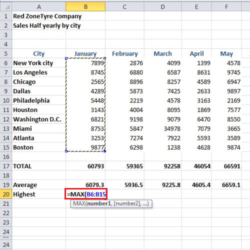
You can even calculate the highest sales that took place in the month of January using a function provided by MS Excel. Under the “average” cell, type “highest” to signify that the highest value is being shown. In the cell next to it, type “=max(B6:B15)” and press the “enter” key once done. Use the “auto fill” option and fill in the rest of the cells .By doing so, you will get to know what the highest value of sales achieved in every month amounted to.
Step # 3 – Calculating the minimum value
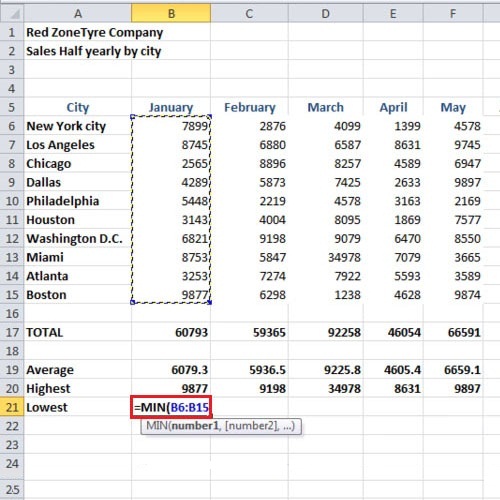
Just as we have calculated the maximum level of sales for each month for the excel column numbers, we can similarly calculate the minimum level of sales. Type “lowest” and in the cell next to it, write “=min(b6:b15)”. Now press the “enter” key. You can now use the “auto fill” option to calculate the same for the rest of the months.
Step # 4 – Calculating the total number of values
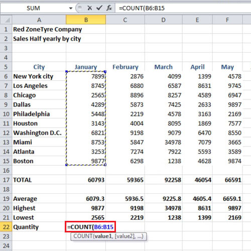
Moreover, you can use another function while working in Excel in order to find out the total number of values that are being used in the calculations. In order to do so, type “quantity” and in the cell next to it, insert the formula “=count(b6:b15)” and press the “enter” key. Using the same method, you can calculate the quantity for the rest of the months as well.
Step # 5 – Removing values
All calculations in MS Excel are calculated with the reference of cell numbers. If you make any changes in the cell values, the calculated values will be changed accordingly. In this tutorial, we deleted the value in cells “d10”, “f8”, “f11” and “f13” and the average value and quantity values changed as a result. By now, you would have a fair idea of how to use Microsoft excel while working with numbers in columns.
 Home
Home