In this tutorial, we’re going to show you how to create a drop-down list in Excel 2016.
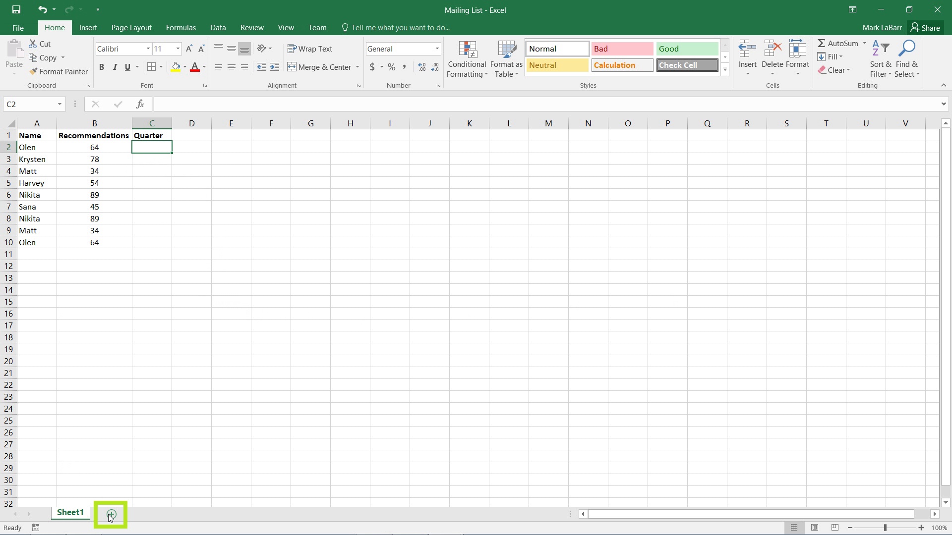
We’ll first create a new Sheet by hitting the plus sign located in the bottom left of the screen.
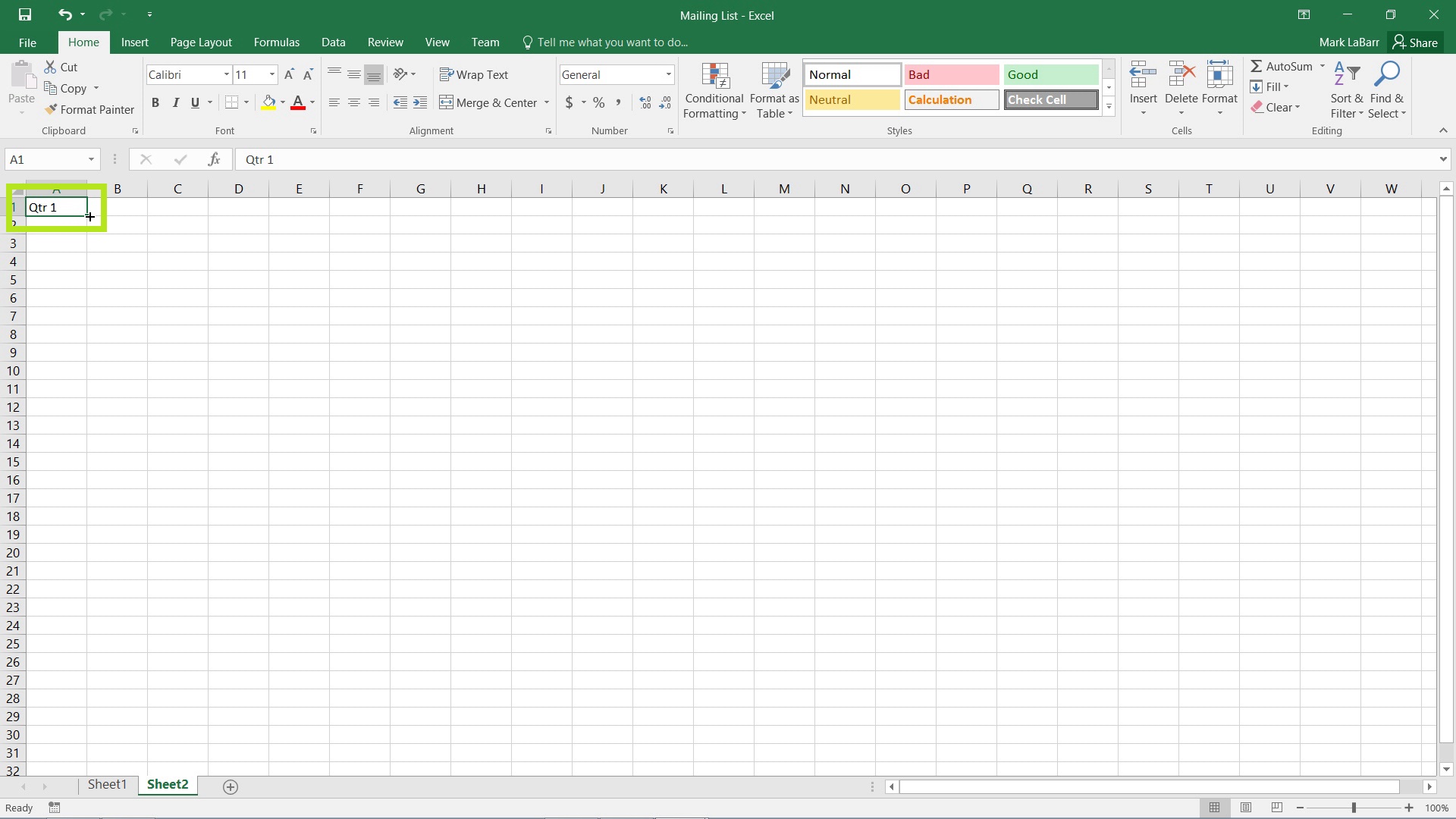
Within this second sheet, we’ll write out the list of options the user can choose within the drop-down list. The example will be numbered, so I will start by typing [Qtr 1] in the first cell. Then, move the cursor to the bottom right of the selected cell until the cursor changes and click and drag it down to however many you want. The list should automatically be numbered.
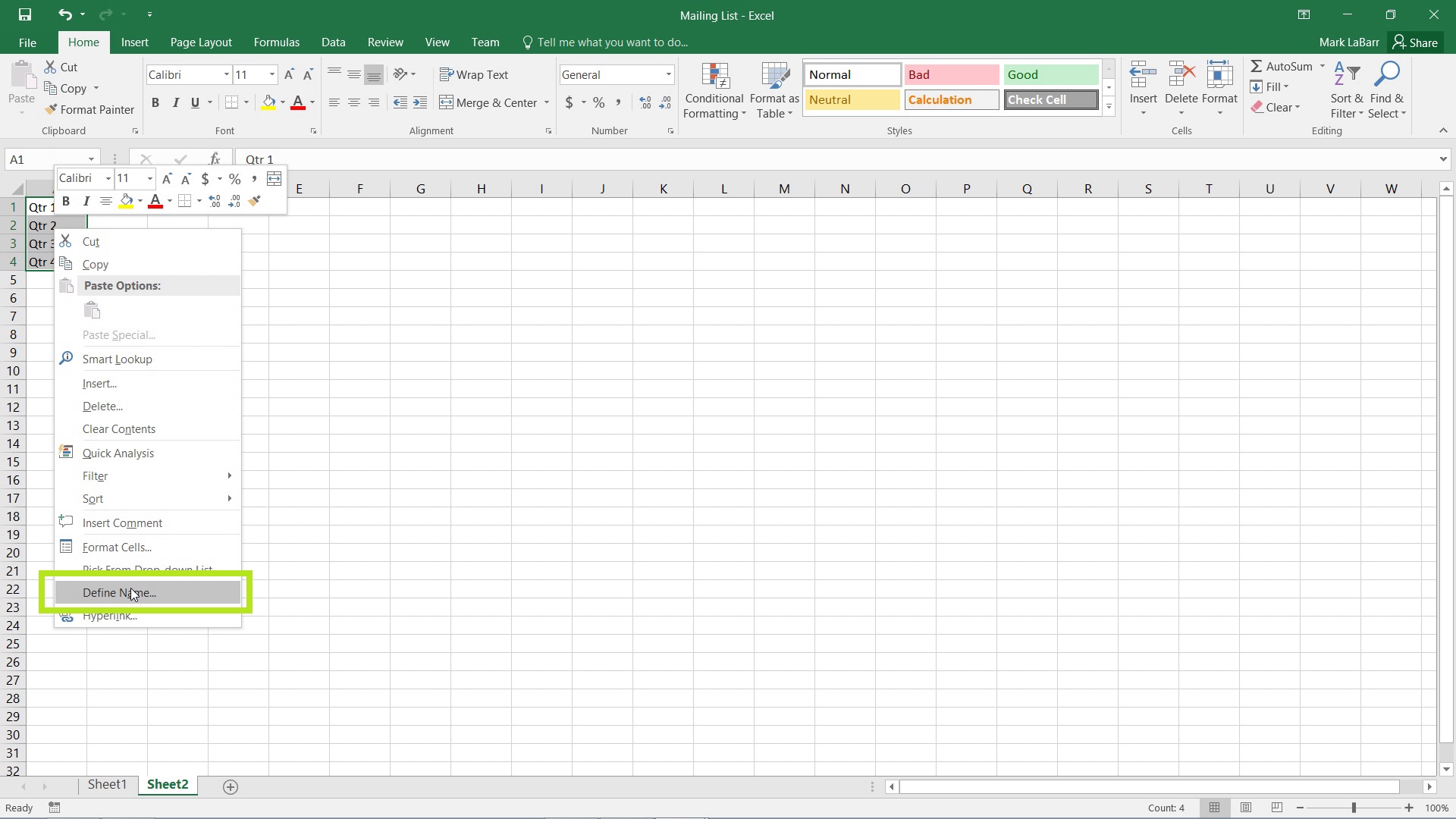
Select the entire list and right-click it. Choose Define Name…
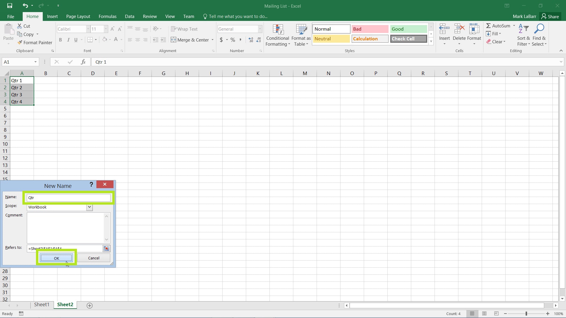
Create a name for the list and remember it. Leave the Scope set to Workbook to allow the list to be used in different Sheets.
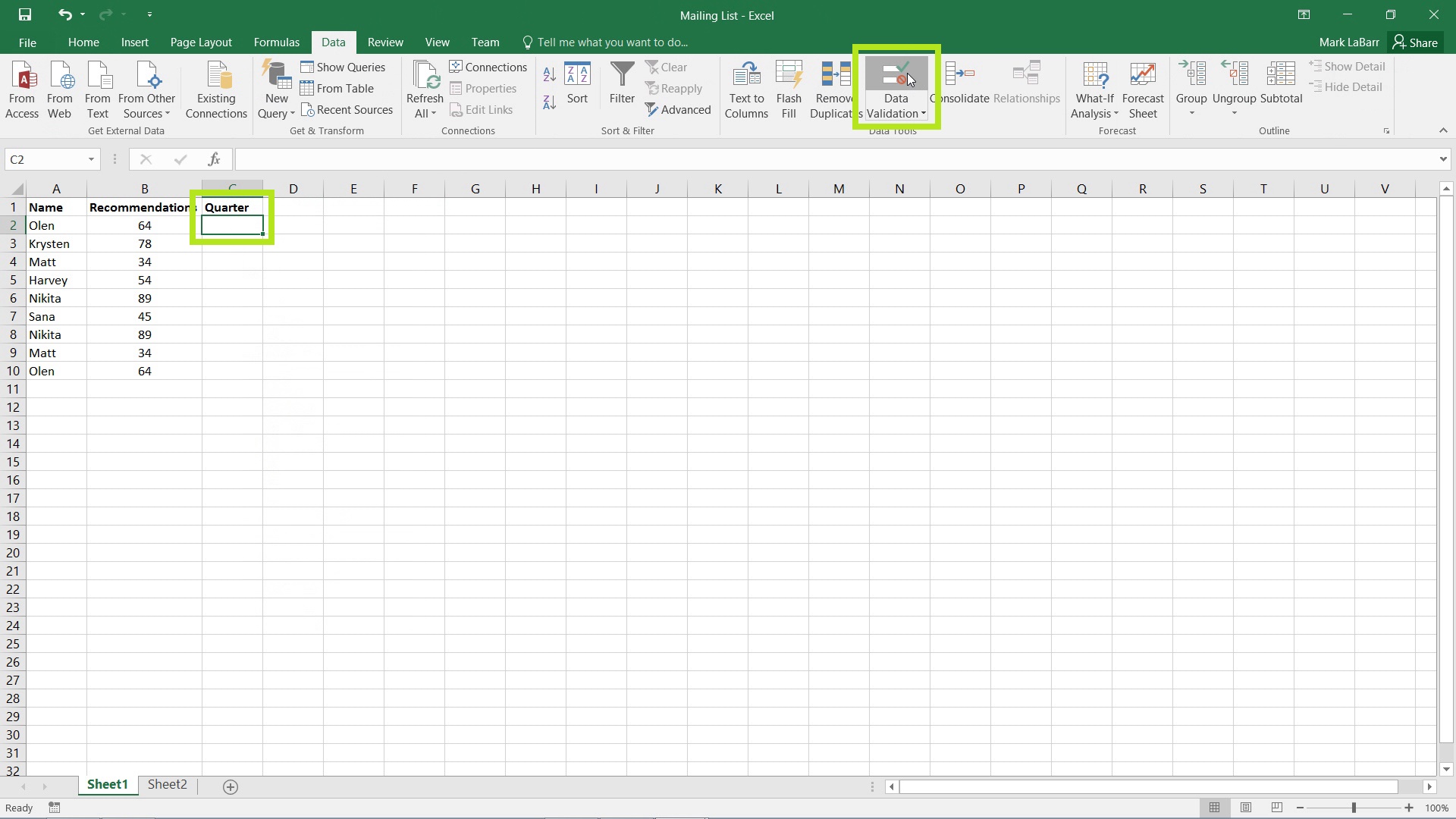
Go back to Sheet 1 and select the first cell you want the drop-down list to be in. Go to the Data tab and click Data Validation.
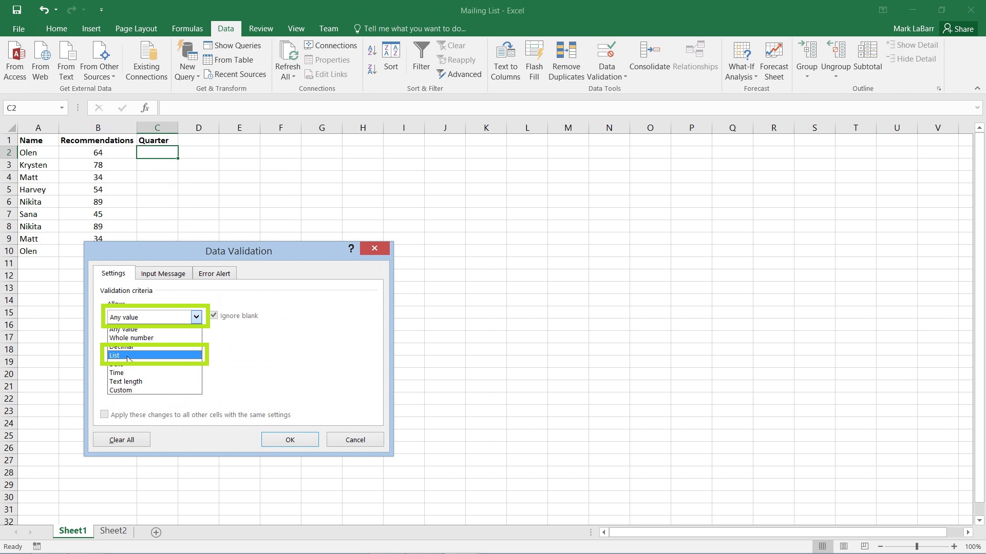
Open the drop-down Allow:, and choose List.
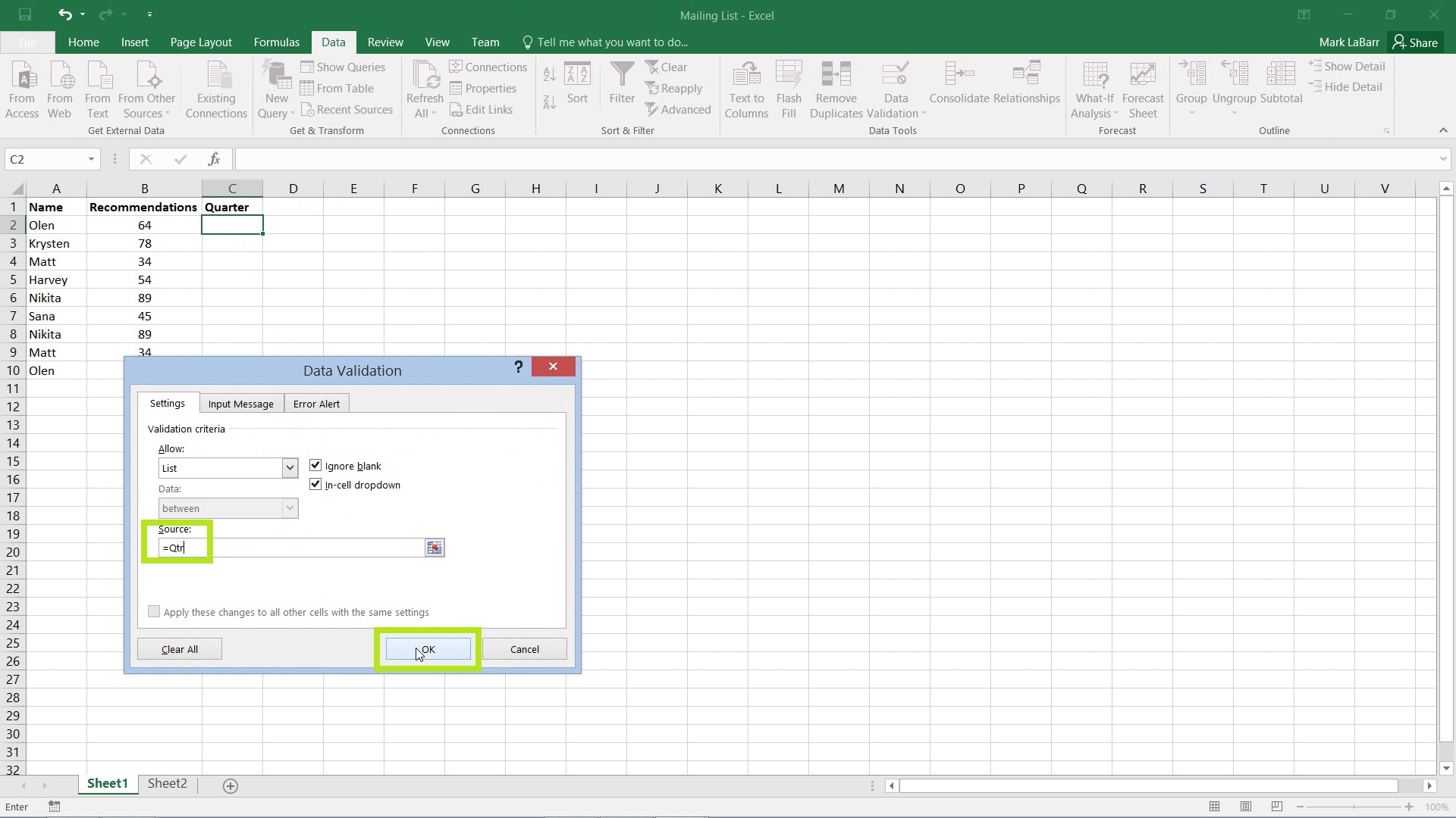
In the Source area, type in the equals (=) sign followed by whatever you named your drop-down. Finally, hit OK.
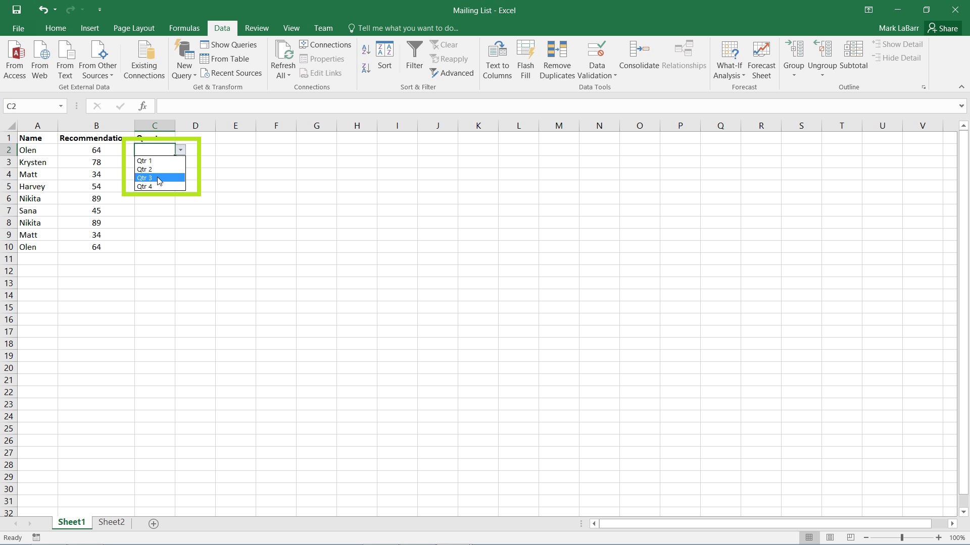
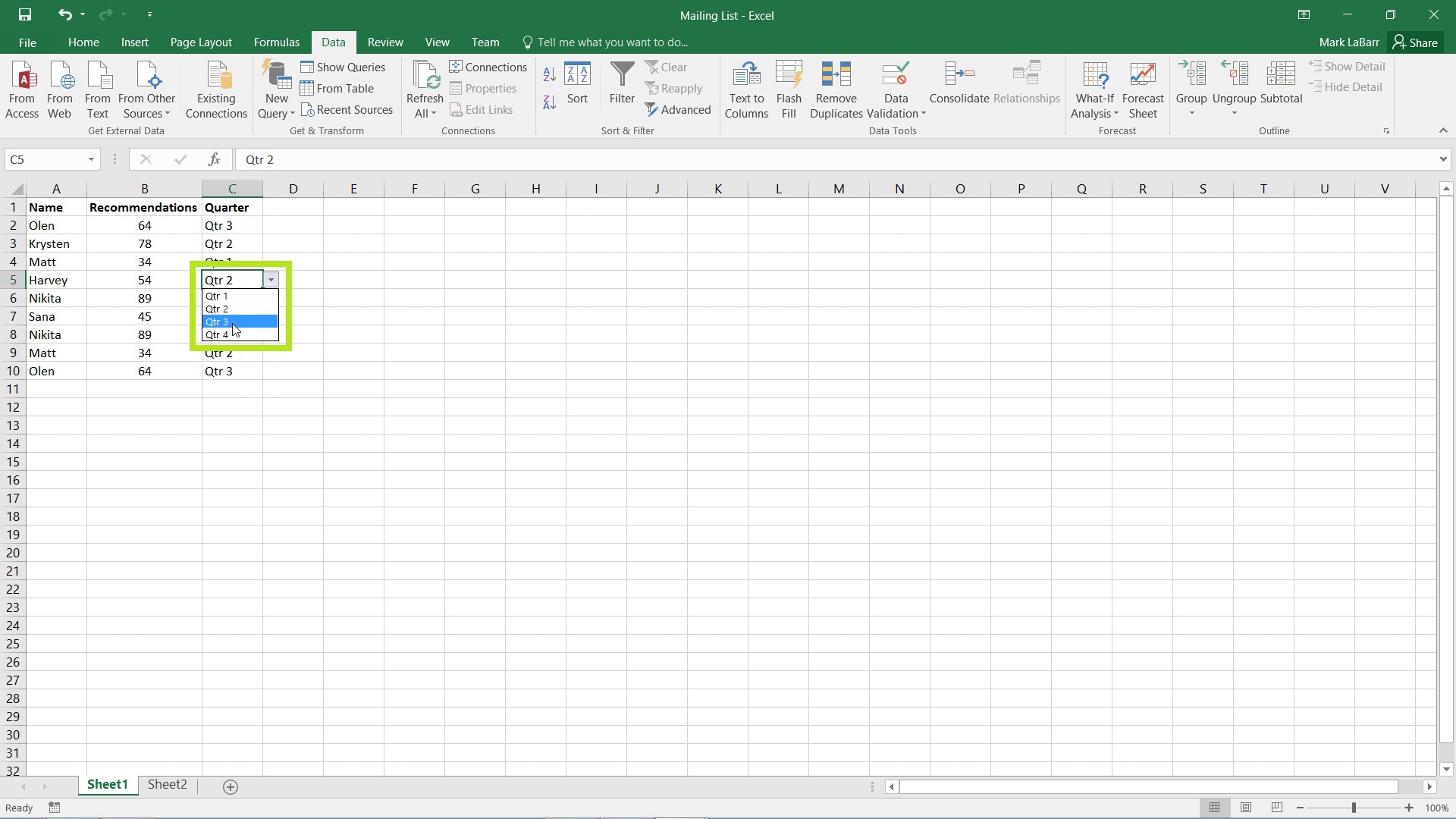
You should now have the option to open the drop-down list of the cell and choose one of the options.
You can copy and paste this cell to other areas of the worksheet, and you can also move your cursor to the bottom right of the selected cell until it changes, and click and drag it to duplicate the contents to all selected cells.
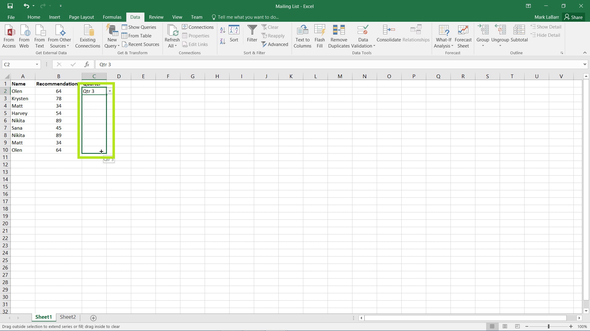
You should now have drop-down capabilities in affected cells.
 Home
Home